MEAN VALUE OF A FUNCTION OF

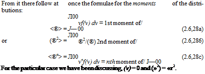
Let g(v) be any function of v. Then if we calculate all the values gn associated with all the samples vn(tj) referred to above we can obtain the ensemble

mean (g). Now it is clear that of all the samples the fraction that falls in the infinitesimal range gi <g <9i + Ag corresponding to the range of v vt < v <: v{■ + Av is f(vt) Av. If now we divide the whole range of g into such equal intervals Ag the mean of g is clearly

00

(g) = lim 2,g(f(v{)Av

A u-*0£=l

or (g) = Г g(v)f(v) dv (2.6,27)

J—oo

Equation (2.6,27) is of fundamental importance in the theory of probability.

JOINT PROBABILITY

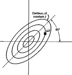
Let vflt) and v2(t) be two random variables, with probability distributions fi(vi) and f2(v2). The joint probability distribution is denoted f(vlt v2), and is defined like f(v). Thus /(iq, v2) AS is the fraction of an infinite ensemble of pairs («j, v2) that fall in the area AS of the vv v2 plane (see Fig. 2.9). If vx and v2 are independent variables, i. e. if the probability j(vx) is not dependent in any way on v2, and vice versa, the joint probability is simply the product of the separate probabilities

/(®i> 4) =/iW/aK) (2.6,29)

From the theorem for the mean, (2.6,27) the correlation of two variables can he related to the joint probability. Thus

B12 = (Vlv2) =jjv1v2f(v1, v2) dvx dv2

— 00

For independent variables, we may use (2.6,29) in (2.6,30) to get

Л oo л oo

^12 = »i/(®i) dv і X V, f(v2) dv,

J— 00 J—oo

= <®l)(®2>

V2

Fig. 2.9 Bivariate distribution.

and is zero if either variable has a zero mean. Thus statistical independence imphes zero correlation, although the reverse in not generally true.

The general form for the joint probability of variables that are separately normally distributed, and that are not necessarily independent is

(2.6,31)

M = [»%]

ma = («л)

N = [»и] = M-i

For two variables this yields the bivariate normal distribution for which

M

As shown in Fig. 2.9, the principal axes of the figure formed by the contours of constant / for given R(t) are inclined at 45°. The contours themselves are ellipses.

JOINT DISTRIBUTION OF A FUNCTION AND ITS SLOPE

We shall require the joint distribution function f(v, v; 0) for a function v(t) that has a normal distribution. The correlation of v and v is

Evv(t) = Ит ^ f v(t)v(t + t) dt

In particular, when т = 0

1 ҐT A;

л*(0) = lim ^ vJ7dt r-co 2T J-t dt

which is zero for a finite stationary variable. It follows therefore from (2.6,33) that f(v, v; 0) reduces to the product form of two statistically independent functions, i. e.

/(»,»; 0) = fx{v) – fiiv)

To evaluate / we need only the two variances. ax = V we have pointed out previously can be found from either i? u(r) or <£>u(ft>). To find a2 = ii we have recourse to the spectral representation (2.6,4), from which it follows that

Л CO

v(t) = imei<oidc (2.6,37)

J CO——CO

From this we deduce that the complex amplitude of a spectral component of v is ico times the amplitude of the same component of v. From (2.6,15) it then follows that the spectrum function for v is related to that for v by

and finally that

(Т22 = (й2) = Ф#(®) dm = (о2Фот(со) dm (2.6,39)

J—CO J—СО

Thus it appears that the basic information required in order to calculate f(v, v) is the power spectral density of v, Ф„„(со). From it we can get both (■v2) and (v2) and hence f(v, v; 0).

The autocorrelation of v can be related simply to that of v as follows. Consider the derivative of R(t)

±nvv(T) = ^<vmt + T)) dr dr

Since the differential and averaging operations are commutative their order may be interchanged to give

j-j; Rw(t) = (v(t) v(t + t)^>

= (v(t)v(t + t)>

Now let (t + r) = u, so that

-7- ^w(r) = (v(u ~ t)v(u)) dr

We now differentiate again at constant u, to get