Delta Form TF
The “q’’-operator of Equation 2.4 is not like the continuous-time operator d( )/dt. If q is replaced by a “difference operator,’’ which is like a ‘‘derivative,’’ the correspondence between discrete-time and continuous-time system will definitely be better. The delta operator with t as the sampling interval is defined as [12]
8 = (2.6)
t
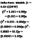
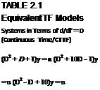
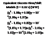
Table 2.1 gives equivalent TF models in various domains: d/dt = D, q or shift form, and delta form.
![]()
|

 |
 |
There is good correspondence between delta form TF (DFTF) and continuoustime system expressions (columns 1 and 3), whereas the correspondence between the continuous-time system and the shift form TF (SFTF; columns 1 and 2) is not obvious, even though these TFs are equivalent in their input/output behavior. The main point is that if we fit a DFTF to the discrete-time data, then from the DFTF we can easily discern the characteristics of the underlying continuous-time system. This cannot be done from SFTF unless it is either converted to discrete Bode diagram or time response is obtained. This is the main advantage of DFTF compared to SFTF.
Similarly DFTF can be converted to CTTF, but it will be seen that the difference between DFTF and CTTF is inherently small and the original DFTF can be interpreted in a manner similar to CTTF, which will not be the case with SFTF in general. We emphasize here that t should be quite small.
In shift form we have
qx(k) = Fx(k) + Gu(k) y(k) = H x(k)
Then in the delta form we have
q = 1 + t5
5x = F’x + G’u (2.7)
y = H x
With
F’ = (F – I)/t; G’ = G/t; H = H
Example 2.5
Obtain the roots of the numerator (zeros) and the denominator (poles) of the model forms [12] given in Table 2.1.
Solution
The zeros and the poles are obtained by using roots ([1 1 1]), etc., as given in Table 2.2. Thus, we see a striking similarity between the poles of CTTF (rows 1, 2, 3) and DFTF (rows 7,8,9), respectively. However, the SFTFs have additionally one zero each, and there is no correspondence between poles of CTTF and SFTF. Thus, one can easily see the merits of DFTFs.
|
TABLE 2.2 Zeros and Poles of the Equivalent TF Models Systems in Terms of d/df = D
|


