Fourth-Order Approximation

If the fourth-order approximation of Eq. (1.23) is used instead of Eq. (1.22), it is easy to show that the governing finite difference equation for йе is

The two physical boundary conditions of Eq. (1.15) are

й0 = 0, йм = 0. (1.35)

Now, Eq. (1.34) is a fourth-order finite difference equation. There are four linearly independent solutions. In order to have a unique solution, four boundary conditions are necessary. However, only two physical boundary conditions are available. To ensure a unique solution of the fourth-order finite difference equation, two extra (nonphysical) boundary conditions need to be created. Also, two of the four solutions of Eq. (1.34) are spurious solutions unrelated to the physical problem. Therefore, the use of high-order approximation will result in

(A) Possible generation of spurious numerical solutions.

(B) A need for extra boundary conditions or special boundary treatment.

These are definite disadvantages in the use of a high-order scheme to approximate partial differential equations. Are there any advantages? To show that there could be an advantage, note that the eigenfunction of the finite difference equation (1.33) is identical to the exact eigenfunction (1.21). As it turns out, the eigenfunction (1.33)

Figure 1.3. Comparison of normal mode

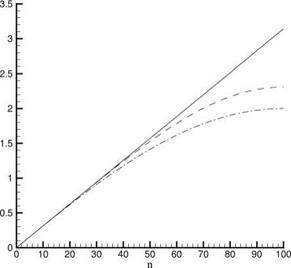frequencies. _________ , exact, Eq.

(1.20);————– , fourth-order, Eq.

(1.37);…… , second-order, Eq. (1.32).

of the second-order approximation is also the eigenfunction of the fourth-order approximation, namely, the solution of Eqs. (1.34) and (1.35) is

Щ = sin( , n = 1 2, 3,…. (1.36)

These eigenfunctions satisfy boundary conditions (1.35). On the substitution of solu­tion (1.36) into Eq. (1.34), it is easy to find that the corresponding eigenfrequency is given by

It is straightforward to find that frequency formula (1.37) is a much improved approximation to the exact eigenfrequency of formula (1.20) than formula (1.32) of the second-order method. Figure 1.3 shows a comparison for the case M = 100. This result illustrates the fact that, when the problems of spurious waves and extra boundary conditions are adequately taken care of, a high-order method does give more accurate numerical results.