State-Space Models

In the modern control/system theory, dynamic systems are described by the state- space representation. Besides the input and output variables, the system’s model has internal states. These models are in time-domain and can be used to represent linear, nonlinear, continuous-time, and discrete time systems with almost equal ease and are applicable to SISO as well as multiple-input multiple-output (MIMO) systems. State-space models are very conveniently used in the design and analysis of control systems. They are mathematically tractable for a variety of optimization, system identification, parameter estimation, state estimation, simulation, and control analysis/design problems. TF models can be obtained easily from state-space models, and they will be unique because TF is the input/output behavior of a system. However, the state-space model from the TF model may not be unique, since the states are not necessarily unique. This means that internal states could be defined in several ways, but the system’s TF from those state-space models would be unique. By definition, the state of a system at any time t is a minimum set of values x1,…, xn, which along with the input to the system for all time T, T > t is sufficient to determine the behavior of the system for all (future) T > t. In order to arrive at the solution to an n-order differential equation completely, we must prescribe n initial conditions at the initial time “t0” and the forcing function for all (future times) T > t0 of interest: n quantities are required to establish the system ‘‘state’’ at t0. However, t0 can be any time of interest, so one can see that n variables are required to establish the state at any given time.

Let a second-order differential equation be given as

Let z(t) ! output

And z(t) = x1 and Z(t) = x2 be the two ‘‘states’’ of the system. Then from Equation 2.8 we have

X1 = Z (t) = x2

X2 = Z(t) = u(t) — 01×2 — «0x1 In vector/matrix form this set can be written as

In compact form we have

x = Ax + Bu; z = Cx (2.10)

with appropriate equivalence between Equations 2.9 and 2.10. The part of Equation 2.10 without the Bu term is called the homogeneous equation.

Example 2.6

Let the state-space model of a system have the following matrices [2]:

	-2 0 1		1
A =	1 -2 0	; в =	0	; C = [2 1 – 1]
	1 1 -1		1

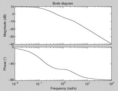
Obtain the TF of this system as well as the Bode diagram.

Solution

Use the function [num, den] = ss2tf([-2 0 1; 1 -2 0; 1 1 -1], [1 0 1], [2 1 -1], [0], 1) to obtain num = [0 1.0 4.0 3.0] and den = [1.0 5.0 7.0 1.0] and hence the following TF can be easily formed:

s2 + 4 s + 3
s3 + 5s2 + 7s + 1

The Bode diagram is obtained as in Example 2.1 (see Figure 2.9). We see that the Bode diagram of this seemingly three degrees of freedom (3DOF) system looks like that of a first-order system. To understand the reason we obtain the roots of the denominator as -2.4196 + 0.6063І; -2.4196 — 0.6063І; -0.1607 and the roots of the numerator as —3.0 and -1.0. Although there is no exact cancellation of the (numerator) zero at 3.0 and the (denominator) complex pole, effectively the frequency response degenerates to that of a TF with reduced order. The eigenvalues of the system obtained by eig(A) are exactly

FIGURE 2.9 Bode plot of the 3DOF state-space system.

the roots of the denominator. This example illustrates a fundamental equivalence between SISO TF and the state-space representation of a dynamic system as well as effective (though not exact) zero/pole cancellation of the TF. This example also hints at the prospect that lower-order equivalent TFs can be obtained from some higher-order TFs by some approximation methods as long as the overall frequency responses (as represented by Bode diagram) and time responses are equivalent in the range of interest.