The Transmission Problem

Consider a plane acoustic wave of angular frequency ы incident on the interface at an angle of incidence в as shown in Figure 1.4. The appropriate solution of Eqs. (1.38) to (1.40) may be written in the following form:

(1.47)

where A is the amplitude and Re{} is the real part of. The reflected wave in region (1) has a form similar to Eq. (1.47), which may be written as

(1.48)

where R is the amplitude of the reflected wave. The transmitted wave in region (2) must have the same dependence on x and t as the incidence wave. Let

(1.49)

a® a(1)

By substituting Eq. (1.49) into Eqs. (1.41) to (1.43), it is easy to find after some simple elimination,

On solving Eq. (1.50), the transmitted wave with an amplitude T may be written as

(2) (2) p(2)

	г sin в -|
T	P(2)a(1) [1—(a(2)/a(1))2 sin2 в ]2/2	e—i®(sin в x+(a(1)/a(2))[1—(a(2)/a(1))2 sin2 в]1/2у+а(1) t}/a(1)
P(2)a(2)
	1

transmitted

= Re

9v(2) _ 1 9p(2)

cos в cos в (1 – (a(2)/a(1)}2sin2 в))1^ A + R = poi®

It is easy to eliminate n(1) and v(1) from Eqs. (1.38) to (1.40) to obtain a single equation for p(1),

Я 2 p(1) d-P— – (i(1))2

d 2 p(1) 9 2 p(1) +

dt2 у dx2 9y2 Once p(1) is found, v(1) may be calculated by Eq. (1.39) or 9 v(1) 1 9 p(1) 91 p(1) 9y ‘ These equations are valid for y > 0. Similarly for y < 0, the equations are

dt p(2) 9 y

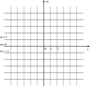
A rectangular mesh with mesh size Ax and Ay, as shown in Figure 1.5, will be used for the finite difference model. Let I and m be the mesh indices in the x and y directions. The fluid interface is at m = 0.

The time dependence of all variables is in the form e-lmt. This may be factored out from the problem. For simplicity, let

ui1m (t)=Re{ pp е-ш (1.60)

(D(1) – 2 f>(1) + D(1) pt+1,m 2p l, m + pl-1,m J

and similarly for all the other variables. Suppose the standard second-order central difference is used to approximate the spatial derivatives in Eqs. (1.56) to (1.59), it is straightforward to obtain

+ 1 (nd) – 2 f,(1) + nd) ^

+ (Ay)2 lm+1 2pl, m + pl, m-1)

1 »(1) – P(1) (1) 1 pl, m+1 pl, m—1

Figure 1.5. Computation mesh.
(1.62)
+ — d(2) — 2 d(2) + d(2) + (Ay)2 Pl, m+1 2 pl, m + pl, m—1
= 0	(1.63)
(1.64)

Now, because a 3-point central difference stencil is used, Eqs. (1.61) and (1.62) should be applicable to values of m > 1. However, if it is insisted that they are to hold true at m = 0, just above the interface discontinuity, then a problem arises. These equations will include the nonphysical variable pf— 1. Similarly, Eqs. (1.63) and (1.64) should be applicable to m < -1. But if they are to be satisfied at m = 0, just below the interface discontinuity, then there is the problem of nonphysical variable pfl appearing in the equations. pf— 1 and p® will be referred to as ghost values and the corresponding row of points at m = — 1 and m = +1 are the ghost points. In a time – domain computation, the values pf ‘0 , v^O are given by the time marching scheme of Eqs. (1.61) and (1.62). Similarly, pfO and v(20 are given by those of Eqs. (1.63) and (1.64). Boundary conditions (1.44) and (1.45), however, require the continuity of pressure and vertical velocity component at the interface. This would not be possible in general. Here, it is important to recognize that, although the pressure is continuous at the interface, the pressure gradient is not. In fact, the pressure gradient should be discontinuous. The jump at the discontinuity is determined by boundary conditions (1.44) and (1.45). In the finite difference model, one may accept pf—1 and p® , the ghost values, as the variables controlling the pressure gradients. These ghost values

of pressure are to be chosen such that the discretized version of boundary conditions (1.44) and (1.45), namely,

f(1) – f ® p 1,0 — p,0

yd) — y(2)

v 1,0 — vl,0

are satisfied. Notice that there are two boundary conditions. They can be enforced by choosing the two ghost values properly.

The finite difference model of sound transmission as formulated, consisting of Eqs. (1.61) to (1.66), can be solved exactly analytically. The exact solution may be found as follows.

The incoming wave at an angle of incidence в and having a total wave number к may be written in the form

p(incoming) ^^/k(sinвДхІ+cosвДym)

2(a(1))2

cos(k sin в Ax) + cos(k cos вДу)
&
— 0. (1.68)
+
(Ax)2	(Ay)2

The cosine functions are symmetric with respect to к, so that if к is a positive real root, then – к is also a root. The positive real root is the total wave number of the incident wave. If & is complex, then к is also complex. It is to be determined by analytic continuation in the complex plane. The reflected wave has the same dependence on I but propagates in the positive m direction. It is straightforward to find that the total wave field in region (1), being the sum of the incident and the reflected waves, may be written as

p(l) Ae_ ‘к (sin eAxl+cos eAym) + Rg_’^(sin eAxl—cos eAym)

(m — 0,1, 2,…).

R is the reflected wave amplitude. By substituting Eq. (1.69) into Eq. (1.62), the vertical velocity component is found, as follows:

5Іп(кcoseAy) г Ag—^(sineAxl+coseAym) + r ^Ік(— sineAxl+coseAym)] m 12 3

&p(1)Ay L ’ ’ ’ * ‘

2&p(1) Ay

Де_ік($тeAxl+coseAy) + r ^’к(_ sineAxl+cos eAy) p(1)

m — 0

(1.70)

The transmitted wave in region (2) must have the same dependence on I as the incident and reflected waves. Thus, let

f.(2) 7^ „_ік sin в Axl—ів Aym

pl, m —

(m — 0, _ 1, _ 2, _ 3,…).

The transmitted wave must satisfy (1.63). On substituting (1.71) into (1.63), it is found that the equation is satisfied if в is the root of

For the outgoing wave, в is the positive real root. If ш is complex, then в is obtained by analytic continuation.

The vertical velocity component of the transmitted wave is given by the substi­tution of (1.71) into (1.64). This yields

It should be obvious that the ghost value of pressure must have the same dependence on I as the incident, reflected, and transmitted waves. Hence, we may write

^(1) ^ ,,—iksineAxl

pl, —1 = p— 1Є

^(2) ^ „—iksineAxl

pl,1 = p1e.

(p(1) — 2p(1) + p(1) ) + 1 (p(1) — 2p(1) + p(1) ) = 0 2 VP£+1,0 2p 1,0 + pl—1,0/ + / л,,л2 VP£1 2p 1,0 + p£ — 1/ = 0

There are four boundary conditions that need to be satisfied at m = 0. The first two are from Eqs. (1.61) and (1.63). By setting m = 0, these equations give

(1.76)

The other two boundary conditions are the dynamic and kinematic boundary con­ditions (1.65) and (1.66). The incident, reflected, and transmitted wave solutions as found consist of Eqs. (1.69), (1.70), (1.71), and (1.73). There are four constants in the solution; they are R, T , p—1 , and p 1 . By substituting the solution into the four boundary conditions, it is straightforward to find that the transmitted and reflected wave amplitudes are given by

T _ 2

A 1 + і р^ 1 sin (в Ay)

+ ур(2) / sin(k cos eAy)

R = T — A.

It is easy to show that, in the limit Ax, Ay ^ 0, k ^ ш/а(1), в ^ ш/а(2) [1 — (р(1)/р(2)) sin2 в]1/2, so that Eq. (1.78) is identical to the exact solution (1.54) of the continuous model.

Figure 1.6 shows the transmitted wave amplitude computed by Eq. (1.78) for the case р(1)/р(2) = 1.2 with &>Ax/a(1) = n/6 and n/4, Ax = Ay as a function of the angle of incidence. There is good agreement with the exact solution (1.54). For the given density ratio, total internal refraction occurs at в = 65.91°. For an

Figure 1.6. Transmitted wave amplitude as a function of the angle of inci­dence. , exact solution; ,

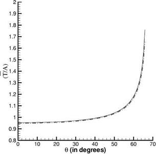&>Ax/a(1) = n/6;….. , &>Ax/a(1) = n/4.

incident angle greater than this value, the incident wave is totally reflected at the interface and there is no transmitted wave. Tbecomes complex, and the transmitted wave becomes damped exponentially in the negative y direction. The cutoff angle as determined by Eq. (1.78) is found to be very close to the exact value.