ANN MODELING

Computationally neural nets are a radically new approach to problem solving. The methodology can be contrasted with the traditional approach to artificial intelligence (AI). Although the origins of AI lay in applying conventional serial-processing techniques to high-level cognitive processing like concept formation, semantics, symbolic processing, etc. (in a top-down approach), the neural nets are designed to take the opposite: the bottom-up approach. The idea is to have a human-like reasoning emerge on the macroscale. The approach itself is inspired by such basic skills of the human brain as its ability to continue functioning with noisy and/or incomplete information, its robustness or fault tolerance, its adaptability to changing environments by learning, etc. Neural nets attempt to mimic and exploit the parallel processing capability of the human brain in order to deal with precisely the kinds of problems that the human brain is well adapted for [16].

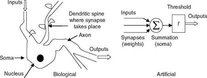
ANNs are new paradigms for computations and modeling of dynamic systems. They are modeled based on the massively parallel (neuro-) biological structures found in brains [16]. ANN simulates a highly interconnected parallel computational structure with relatively simple individual processing elements called neurons. The human brain has 10-500 billion neurons and about 1,000 main modules with 500 NWs and each such NW has 100,000 neurons [16]. The axon of each neuron connects to several hundred or thousand other neurons. The neuron is a basic building block of a nervous system. Comparison of a biological neuron and an ANN is shown in Table 2.3 and Figure 2.13.

The equivalence of the neuron process to an electronic circuit is discussed here. The voltage amplifier simulates a cell body; the wires represent the input (dendrites) and output (axon) structures. The variable resistors model the synaptic weights and the sigmoid function is the saturation characteristic of the amplifier. It is apparent from the foregoing that, for ANN, a part of the behavior of real neurons is used and ANN can be regarded as multi-input nonlinear device with weighted connections. The cell body is a nonlinear limiting function, an activation step (hard) limiter (for logic circuit simulation/modeling), or an S-shaped sigmoid function for general modeling of nonlinear systems.

TABLE 2.3

Biological and Artificial Neuronal Systems

Artificial Neuronal System

• Data enter the input layer of the ANN

• One hidden layer is between input and output layers; one layer is normally sufficient

• Output layer that produces the NW’s output responses can be linear or nonlinear

• Weights are the strength of the connection between nodes

Biological Neuronal System

* Dendrites are the input branches—tree of fibers and connect to a set of other neurons—the receptive surfaces for input signals

* Soma cell body wherein all the logical functions of the neurons are performed

* Axon nerve fiber—output channel, the signals are converted into nerve pulses (spikes) to target cells

* Synapses are the specialized contacts on a neuron, and interface some axons to the spines of the input dendrites; can enhance/dampen the neuron excitation

ANNs have found successful applications in image processing, pattern recogni­tion, nonlinear curve fitting/mapping, flight data analysis, adaptive control, system identification, and parameter estimation. In many such cases ANNs are used for prediction of the phenomena that they have learnt earlier by way of training from the known samples of data. They have good ability to learn adaptively from the data. The specialized features that motivate the strong interest in ANNs are as follows:

1. NW expansion is a basis (recall Fourier expansion/orthogonal functions as basis for expression of time-series data/periodic signals).

2. NW structure extrapolates in adaptively chosen directions.

3. NW structure uses adaptive bases functions—the shape and location of these functions are adjusted by the observed data.

neuron neuronal model

4. NW’s approximation capability is good.

5. NW structure is repetitive in nature and has advantage in HW/SW imple­mentations.

6. This repetitive structure provides resilience to failures. The regularization feature is a useful tool to effectively include only those basic functions that are essential for the approximation and this is achieved implicitly by stopping rules and explicitly by imposing penalty for parameter deviation.

Conventional computers based on Von Neumann’s architecture cannot match the human brain’s capacity for several tasks like: (1) speech processing, (2) image processing, (3) pattern recognition, (4) heuristic reasoning, and (5) universal problem solving. The main reason for this capability of the brain is that each biological neuron is connected to about 10,000 other neurons and this in turn gives it a massively parallel computing capability. The brain effectively solves certain prob­lems that have two main characteristics: (1) these problems are generally ill-defined and (2) they usually require a large amount of processing. The primary similarity between the biological nervous system and ANN is that each system typically consists of a large number of simple elements that learn and are collectively able to solve complicated and ambiguous problems. It seems that a ‘‘huge’’ amount of ‘‘simplicity’’ rules the roost.

Computations based on ANNs can be regarded as ‘‘sixth-generation computing’’ or as a kind of extension of massively parallel processing (MPP) of ‘‘fifth-generation computing’’ [17]. MPP super computers give higher throughput per money value than conventional computers for the algorithms within the domain of programming constraints of such computers. ANNs can be considered as any general-purpose algorithm within the constraints of such sixth-generation hardware. The human brain lives within essentially the same sort of constraints. ANN applications for large and more complex problems become more interesting. One can develop new generations of ANN design providing new learning-based capabilities in control and system identification. These new designs could be characterized as extensions or as an aid to existing control theory and new general control designs compatible with ANN implementation. One can exploit the power of new ANN chips or optical HW, which extend the ideas of MPP, and reduced instruction sets down to a deeper level permitting orders of magnitudes more throughput per money value.

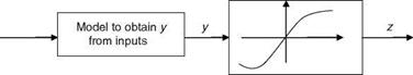
There are mainly two types of neurons used in NWs: sigmoid and binary. In sigmoid neurons the output is a real number. The sigmoid function (see Figure 2.14) often used is

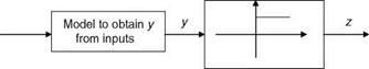
FIGURE 2.15 Binary neuron model.

z = 1/(1 + exp(-y)) = (1 + tan h(y/2))/2

y could be a simple linear combination of the input components or it could be the result of some more complicated operations: y = summation of (weights * x) – bias! y = weighted linear sum of the components of the input vector and the threshold. In a binary neuron the nonlinear function (see Figure 2.15) is

z = saturation(y) = {1 if y >= 0} and {0 if y < 0}.

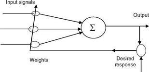
Here also, y could be a simple linear combination of the input components or it could be the result of more complicated operations. The binary neuron has saturation/hard nonlinear function. This type of binary neuron is called a peceptron. One can have a higher-order perceptron where the input y is a second-order polynomial (as a function of input data). A basic building block of most ANNs and adaptive circuits is the adaptive linear combiner (ALC) shown in Figure 2.16. The inputs are weighted by a set of coefficients and the ALC outputs a linear combination of inputs. For training, the measured input patterns/signals and desired responses are presented to the ALC. The weight adaptation is done using the LMS algorithm (Widrow-Hoff delta rule), which minimizes the sum of squares of the linear errors over the training set [18]. More useful ANNs have MLPNs with an input layer, one or at most two hidden layers and an output layer with sigmoid (nonbinary) neuron in each layer. In this NW, the input/output are real-valued signals/data. The output of MLPN is a differential function of the NW parameters. This NW is capable of approximating arbitrary nonlinear mapping using a given set of examples. For a fully connected

Inputs

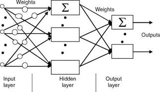FIGURE 2.17 FFNN topology.

MLPN, 2-3 layers are generally sufficient. The number of hidden layer nodes should be much less than the number of training samples. An important property of the NW is the generalization property, which is a measure of how well the NW performs on actual problems once training is completed. Generalization is influenced by the number of data samples, the complexity of the underlying problem, and the NW size.