Boundary Modes

It turns out that the discretized interface problem consisting of finite difference equations (1.61) to (1.64) and boundary conditions (1.65) and (1.66) supported nontrivial homogeneous solutions. These are eigensolutions. They will be referred to as boundary modes. These solutions are bounded spatially, but they may grow or decay in time. A numerical solution is stable only if all boundary modes decay in time. If there is one growing boundary mode, then, in time, this mode will dominate the entire solution leading to numerical instability.

To find the boundary modes, let them be of the form,

pfl = AeiaiAx+ie1mAy, m = -1, 0,1, 2,… (1.80)

p® = BeiaiAx-ie2mAy, m = 1, 0, – 1, – 2,… (1.81)

where a, the wave number, is real and arbitrary. вi and в2 may be complex. For spatially bounded boundary modes, it is required that

Im(e1) > 0; Im(e2) > 0. (1.82)

IfIm(e1 )= 0,thenRe(e1 )> 0 and, similarly, if Im(e2 )= 0,thenRe(e2 )> 0 to satisfy the outgoing wave condition.

Substitution of Eq. (1.80) into Eq. (1.61) yields

Similarly, substitution of Eq. (1.81) into Eq. (1.63) leads to

The corresponding v{pm and vf^ may easily be found by solving Eqs. (1.62) and (1.64). They are found to be

,2(1) = Л 8ш(в1Ду> еіаІДх+і0,тДу vl, m = A -(1Ь Є

шр(1> Ду

д(2> ЕрШ(в2Ду> ^іаІДх-ів2тДу

Vl, m = B -(2Ь Є ‘

шр(2> Ду

Upon imposing the dynamic and kinematic boundary condition (1.65) and (1.66) on solutions (1.80), (1.81), (1.85), and (1.86), it is straightforward to obtain

A – B = 0

For nontrivial solutions, the determinant, D, of the coefficient matrix of the above 2 x 2 linear system for A and B must be equal to zero; i. e.,

The eigenvalues, «Дх/й(1>, of the boundary modes are the roots of Eq. (1.87) for a given аДх.

To determine the eigenvalues numerically, the following grid search method may be used. To start the search, the complex «Дх/а(1> plane is divided into a grid. The intent is to calculate the complex value of D at each grid point. Once the values of D on the grid are known, a contour plot is used to locate the curves Re(D) = 0 and Im(D) = 0 (where Re() and Im() denote the real and imaginary part). The intersections of these curves give D = 0 or the locations of the boundary mode frequencies. To improve accuracy, one may use a refined grid or use a Newton or similar iteration method.

To calculate the value of D at a grid point in the complex «Дх/а(1> plane for a prescribed density and mesh size ratio and аДх, the values of в 1Ду and в2Ду are first computed by solving Eqs. (1.83) and (1.84). All these values are then substituted into Eq. (1.87) to compute D. Figure 1.7 shows the contours Re(D) = 0 and Im(D) = 0 for the case p(1>/p(2> = 2.0 , Дх = Ду, and аДх = n/10. These two curves intercept each other on the real «Дх/а(1> axis at «Дх/а(1> = (0.536, 0.0). Since «Дх/а(1> is real, this root corresponds to a neutral mode. With the addition of artificial selective damping to the finite difference scheme, which is a standard procedure and will be

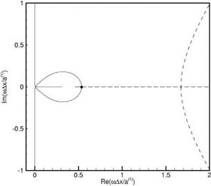Figure 1.7. Location of the roots of D in the complex «Ax/5[1] [2] plane. p(1)/p(2) =

2.0, Ax = Ay, and aA = n/10.———— ,

Re(D) = 0.0;…….. , Im(D) = 0.0.

discussed in a later chapter, the mode will be damped. Thus, the finite difference scheme is not subjected to numerical instability arising from boundary modes.

EXERCISES

where l, m are the spatial indices in the x and y directions (I = 0,1,2,…, N; m = 0, 1,2,…, M). The boundary conditions for the finite difference equations are

at l = 0, l = N, m = 0, m = M, Ul = 0.

l, m

Now, suppose the simple wave equation is discretized by using a second-order central difference approximation. This gives

d2ue c2

~dF = (Xx? (u’+1 _ 1 +111-1

where l is the spatial index.

Consider an incident wave of the form

ut (t) = Ає-і(кІАх+юі

where к Ax = cos-1 (1 – ^2-). Note: the value of к, the wave number, is determined by the requirement that the incident wave satisfies the governing finite difference equation.

Find the reflected wave of the discretized system and show that the reflected wave has the same amplitude as the incident wave. Notice that the wave number к and, hence, the phase velocity, «/к, and group velocity, йш/йк, of the waves supported by the finite difference approximation are not the same as those of the original simple wave equation. Is the approximation good at high or low frequency?

1.3. Acoustic waves in a medium at rest are governed by the linearized Euler and energy equations. Let (u, v) be the velocity components in the x and y directions and p0 and p0 be the static density and pressure. The governing equations are

du 1 d p

+ = 0 d t p0 dx

A +1 dJP = 0

d t P0 dy

where y is the ratio of specific heats. Upon eliminating u and v, it is easy to find that the governing equation for p is

д 2 p = c2 = m

dt2 c дx2 + дy2 ’ c p0

Consider plane acoustic waves propagating at an angle в with respect to the y-axis incident on a wall lying on the x-axis. The incident wave is given by

p = Ae – — (X sin в +y cos в +ct)

p incident Ae

The boundary condition at the wall is

У = о, v = 0.

By the у-momentum equation, the wall boundary condition for pressure p is

At у = 0, — = 0.

У ду

In order to satisfy the wall boundary condition, a reflected wave is generated at the wall. This reflected wave cancels the pressure gradient of the incident wave in the у direction at the wall, namely,

It is easy to find that the solution of Eq. (A) that satisfies Eq. (C) is,

„ _ aJc (-x sin в +у cos в-ct)

preflected

By formulas (B) and (D), it is straightforward to show that the following well-known properties of acoustic wave reflection are true.

(i) The angle of reflection is equal to the angle of incidence.

(ii) The reflected wave has the same intensity as the incident wave.

(iii)

There is a pressure doubling at the wall, that is,

where the overbar denotes a time average.

Suppose the problem is solved by finite difference approximation with a mesh size of Ax and Ду. On using a second-order central difference approximation, Eqs. (A) and (C) become

where l, m are the spatial indices in the x and у directions and the wall is located at m = 0.

Find the incident wave with frequency ю and angle of incidence в. Find the ref­lected wave so that boundary condition (F) is satisfied. Determine whether the acoustic wave reflection properties (i), (ii), and (iii) are satisfied. Would you be able to find the incident and reflected waves if a fourth-order central difference scheme is used?