Schemes with Large Stencils

By now, it is clear that, if one wishes to resolve short waves using a fixed size mesh, it is necessary to use schemes with large stencils. However, there is limitation to this. Beyond the optimized 7-point stencil (n = 1.1) with resolved wave number range up to a Ax = 0.95 (seven mesh spacings per wavelength), it will take a very large increase in the stencil size to improve the resolution to five or four mesh spacings per wavelength. So the cost goes up quite fast.

Consider a very large stencil, say N = 7 or a 15-point stencil. The stencil coefficients can be determined in the same way as before by minimizing the inte­grated error E.

n

E = J a Ax — aAx|2 d (a Ax).

-n

For n = 1.8 (a good overall compromise), the coefficients are

a0 = 0.00000000000000000000000000000 + 0 a3 = —a—1 = 9.1942501110343045059277722885,0 — 1 a2 = —a—2 = —3.55829599268352687556676424010 — 1 a3 = —a—3 = 1.52515016084064924691049286790 — 1 a4 = — a—4 = —5.94630408297157726668285968990 — 2 a5 = —a—5 = 1.90107527095082986598491679880 — 2 a6 = —a—6 = —4.38086492973364818511370009070 — 3 a7 = — a—7 = 5.38961218686233846596929558780 — 4

For comparison purposes, the coefficients of the standard fourteenth-order central difference scheme are

a0 = 0.00000000000000000000000000000 + 0 ax = —a—1 = 8.750000000000000000000000000000 — 1 a2 = —a—2 = —2.91666666666666666666666666670 — 1 a3 = —a—3 = 9.72222222222222222222222222220 — 2 a4 = —a—4 = —2.65151515151515151515151515010 — 2 a5 = —a—5 = 5.3030303030303030303030303030300 — 3 a6 = —a—6 = —6.79875679875679875679875679870 — 4 a7 = —a—7 = 4.16250416250416250416250416250 — 5

The a Ax versus a Ax and the dal da versus a Ax curves are shown in Figures 2.7 and 2.8, respectively. The choice of n is based on the enlarged da/da curve. For very large stencils, these curves exhibit small-amplitude oscillations. The n = 1.8 case gives a good balance between the resolved band width and constancy of group velocity. This stencil can resolve waves as short as 3.5Ax.

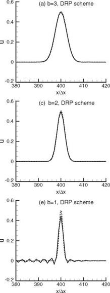
To demonstrate the effectiveness of the use of a large computation stencil to resolve short waves, again consider the initial value problem of Eqs. (2.15) and (2.16). The initial disturbance is again taken to be a Gaussian

f (x) = he— ln2( b)2, (2.23)

Figure 2.7. aAx versus aAx curve for the optimized 15-point stencil (n = 1.8) and the standard fourteenth-order cen­tral difference scheme………………………………………….. , opti­mized scheme; , standard

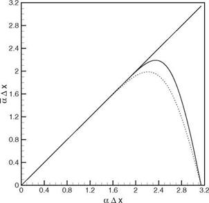fourteenth-order scheme.

where h is the initial maximum amplitude of the pulse and b is the half-width. The Fourier transform of (2.23) is

hb _ а2ь2

f = – г Є 4ln2.

2(n ln2) 2

Notice that the smaller the value of b, the sharper is the pulse waveform in physical space. Also, the corresponding wave number spectrum of the pulse is wider. This makes it more difficult to produce an accurate numerical solution. The numerical results correspond to h = 0.5 and b = 3,2, and 1 using the standard fourteenth-order

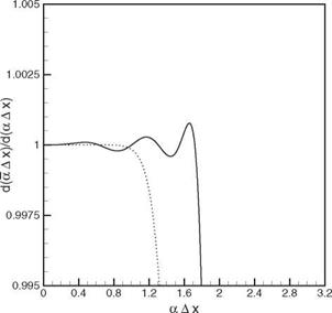Figure 2.8. d(aAX) versus aAx for the

—– 15-point optimized scheme (n =

1.8) and the……… standard fourteenth-

order central difference scheme.

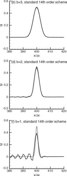Figure 2.9. Comparisons between the computed and the exact solutions of the convective wave equation. t = 400, h = 0.5. Dispersion-relation-preserving scheme is the optimized scheme, exact solution, computed solution.

scheme and the optimized scheme (n = 1.8) are given in Figure 2.9. With b > 2, the optimized scheme gives good waveform. However, for an extremely narrow pulse, b = 1, none of these schemes can provide a solution free of spurious waves.