. Shifting Theorem

Transform of f (x + X) = e>aX f (a).

Now, by applying the Fourier transform to Eq. (2.6) and making use of the Derivative and Shifting theorems, it is found that

where

a on the left of (2.8) is the wave number of the partial derivative. By comparing the left and right sides of this equation, it becomes clear that a on the right side is effectively the wave number of the finite difference scheme. a Ax is a periodic function of a Ax with a period of 2n. To ensure that the Fourier transform of the finite difference scheme is a good approximation of that of the partial derivative over the wave number range of, say, waves with wavelengths longer than four Ax or a Ax < (n/2), it is required that aj be chosen to minimize the integrated error, E, over this wave number range, where

2

E = j |aAx — aAx[3]d (a Ax). (2.10)

— 2

In order that a is real, the coefficients aj must be antisymmetric; i. e.,

a0 = 0, a—j = —aj. (2.11)

On substituting a from Eq. (2.9) into Eq. (2.10) and taking Eq. (2.11) into account, E may be rewritten as,

Eq. (2.13) provides N equations for the N coefficients aj, j = 1,2,…, N. Now consider the case of N = 3 or a 7-point stencil.

There are three coefficients a1, a2, and a3 to be determined. It is possible to combine the truncated Taylor series method and the Fourier transform optimization method.

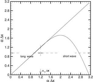
Figure 2.1. a Ax versus a Ax for the 7- point fourth-order optimized central dif­ference scheme.

Let Eq. (2.14) be required to be accurate to O(Ax4). This can be done by expanding the right side of Eq. (2.14) as a Taylor series and then equating terms of order Ax and (Ax)3. This gives

9 4a1

20 – T 2 a1

-15 + У’

On substitution into Eq. (2.12), the integrated error E is a function of a1 alone. The value a1 may be found by solving

— — 0. d ax

This gives the following values

a0 — 0 a1 — —a-1 — 0.79926643

a2 — — a—2 — —0.18941314 a3 — — a—3 — 0.02651995.

The relationship between a Ax and a Ax over the interval 0 to n for the optimized 7-point stencil is shown graphically in Figure 2.1. For a Ax up to about 1.2, the curve is nearly the same as the straight line a Ax — a Ax. Thus, the finite difference scheme can provide reasonably good approximation for a Ax < 1.2 or X > 5.2Ax, where X is the wavelength.

For a Ax greater than 1.6, the a (a) Ax curve deviates increasingly from the straight-line relationship. Thus, the wave propagation characteristics of the short waves of the finite difference scheme are very different from those of the partial differential equation. There is an in-depth discussion of short waves later.

Figure 2.2. d(ffX) versus aAx for N = 3, fourth-order scheme optimized over the range of —n /2 to n/2.