Additive Fuzzy System

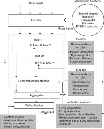
Each input partially fires all rules in parallel and the system acts as an associative processor as it computes the output F(x). The system then combines the partially fired ‘‘then’’ part fuzzy sets in a sum and converts this sum to a scalar or vector output. Thus, a match-and-sum fuzzy approximation can be viewed as a generalized AI expert system or as a (neural-like) fuzzy associative memory. Adaptive fuzzy systems (AFSs) have proven universal approximators for rules, which use fuzzy sets of any shape and are computationally simple. A feedback fuzzy system (rules feedback to one another and to themselves) can model a dynamic system: dx/dt = F(x). The core of every fuzzy controller is the fuzzy inference engine (FIE), the computation mechanism with which decisions can be inferred even though the knowledge may be incomplete. This mechanism gives the linguistic controller the power to reason by being able to extrapolate knowledge and search for rules, which only partially fit any given situation for which a rule does not exist. The FIE performs an exhaustive search of the rules in the knowledge base (rule base) to determine the degree of fit for each rule for a given set of causes (see Figure 2.19). The input and output are crisp variables.

Several rules contribute in varying degrees to the final result. A degree of fit of unit implies that only one rule has fired and only one rule contributes to the final decision; a degree of fit of zero implies that none of the rules contribute to the final decision. The knowledge necessary to control a plant is usually expressed as a set of linguistic rules of the form: If (cause) ‘‘then’’ (effect). These are the rules with
which new operators are trained to control a plant and they constitute the knowledge base of the system. All the rules necessary to control a plant might not be elicited or known. It is therefore essential to use some technique capable of inferring the control action from available rules. FL base control has several merits: (1) for a complex system, a mathematical model is hard to obtain, (2) fuzzy control is a model-free approach, (3) human experts can provide linguistic descriptions about the system and control instructions, (4) fuzzy controllers provide a systematic method to incorporate the knowledge of human experts. The assumptions in an FL control system are as follows: (1) the plant is observable and controllable, (2) expert linguistic rules are available or formulated based on engineering common sense, intuition, or an ana­lytical model, (3) a solution exists, (4) one can look for a good enough solution (approximate reasoning in the sense of probably approximately correct solution, e. g., algorithm) and not necessarily the optimum one, and (5) one can desire to design a controller to the best of our knowledge and within an acceptable precision range. Figure 2.20 depicts a macrolevel computational schematic of the fuzzy inference process: fuzzification (using membership functions), basic operations (on the defined rules), fuzzy implication process (using implication methods), aggregation, and finally defuzzification (using defuzzification methods) [23,24]. Example 2.13 illus­trates the definition of fuzzy membership functions (GMF, TMF, etc.) as seen in Figure 2.21, definition of fuzzy operators, numerical computations to obtain the fuzzy counterpart of the classical intersection and union, and comparison with other such operations. The example requires careful study, but tells us many simple things about fuzzy operators, which are routinely used in modeling and control of dynamic systems. In Chapter 9, we present an FL-based Kalman filter for aircraft state – estimation, whereby other aspects of fuzzy operations would be clear.

Example 2.13

The fuzzy operators corresponding to the well-known Boolean operators AND and OR

are, respectively, defined as min and max [23,24]:

mAnB(u) = mm[mA(u), mB(u)] (intersection)
mAus(“) = max[mA(u), ^b(“)] (union)

FIGURE 2.20 Fuzzy inference system with implication process.

Another method to define AND and OR operators has been proposed by Zadeh [23,24]:

mAns(u) = mA(u)mB(u) (7)

mAus(u) = mA(u) + тв(и) – mA(u)mB(u) (2-38)

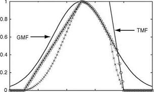
Define fuzzy sets A and B by Gaussian and Trapezoidal membership functions (see GMF, TMF in Figure 2.21) (mA(u), mB(u)), respectively. Obtain the fuzzy intersection (element wise) by placing mA(u) and mB(u) in Equations 2.35 or 2.37. In addition, obtain Fuzzy union (element wise) by using Equations 2.36 or 2.38.

0 2 4 6 8 10

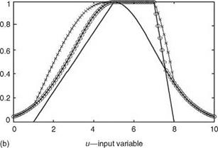
(a) u—input variable FIGURE 2.21 (a) Fuzzy intersection operations (Equation 2.37—x and Equation 2.35—O); (b) fuzzy union operations (Equation 2.38—x and Equation 2.36—O).

Solution

The results are shown in Figure 2.21. Let us denote a — mA(u) and b — mB(u) to be membership grades (within interval [0,1]). Now assume that for some value of input u, a < b; therefore, mAnB(u) using Equation 2.35 will be

mAnB(u) = min (a, b) = a (2.39)

In addition, it is known that b < 1 and multiplying this expression with a gives ab < a. Using Equation 2.37 in the left hand side of ab < a results in ab < min(a, b) which shows that Equation 2.37 < Equation 2.35 (in the sense of the numerical values), i. e., the area covered by x-line (representing Equation 2.37) is lesser than that covered by 0-line (representing Equation 2.35). The same equality holds for a > b. The member­ship function obtained by Equation 2.38 expands compared to the one obtained by Equation 2.36 (Figure 2.21b). This can be easily proved by a numerical example. Let us assume a — 0.1 and b — 0.5 for some value of input variable u. By placing them in

Equations 2.38 and 2.36 we get тлив(и) equal to 0.55 and 0.5 (one can easily verify this), respectively, which means that Equation 2.38 > Equation 2.36, i. e., the area covered by x-line (representing Equation 2.38) is greater than that covered by 0-lines (representing Equation 2.36).

It is apparent from the above definitions that, unlike in crisp logic/set theory, the fuzzy operators can have seemingly different definitions. However, these would be mathematically consistent and would be intuitively valid and appealing [7].

EPILOGUE

Various models for representing dynamic systems have been considered in this chapter. The treatment has been kept as simple as possible. State-space and TF models are very appropriate for parameter estimation and system identification and also useful for evaluating the HQs of aircraft. ANNs and FL find several applications in control, simulation, and modeling [23,25,26]. In Ref. [27], the authors consider the application of NWs for assessing the behavior of the human pilot in the task of maintaining the flight path and airspeed during wind shear approaches. In Ref. [28], fuzzy modeling is proposed for identification, where data are classified by fuzzy clustering and then rules are extracted from these clusters.