Multiple interacting subsystems

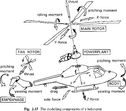
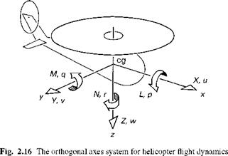
The behaviour of a helicopter in flight can be modelled as the combination of a large number of interacting subsystems. Figure 2.15 highlights the main rotor element, the fuselage, powerplant, flight control system, empennage and tail rotor elements and the resulting forces and moments. Shown in simplified form in Fig. 2.16 is the orthogonal body axes system, fixed at the centre of gravity/mass (cg/cm) of the whole aircraft, about which the aircraft dynamics are referred. Strictly speaking, the cg will move as the rotor blades flap, but we shall assume that the cg is located at the mean position, relative to a particular trim state. The equations governing the behaviour of these interactions are developed from the application of physical laws, e. g., conservation of energy and Newton’s laws of motion, to the individual components, and commonly take the form of nonlinear differential equations written in the first-order vector form

dx

-= f (X, u, t) (2.1)

dt

with initial conditions x(0) = xo.

x (t) is the column vector of state variables; u (t) is the vector of control variables and f is a nonlinear function of the aircraft motion, control inputs and external distur­bances. The reader is directed to Appendix 4A for a brief exposition on the matrix – vector theory used in this and later chapters. For the special case where only the six rigid-body degrees of freedom (DoFs) are considered, the state vector x comprises the three translational velocity components u, v and w, the three rotational velocity components p, q and r and the Euler angles ф, 9 and ф. The three Euler attitude an­gles augment the equations of motion through the kinematic relationship between the

fuselage rates p, q and r and the rates of change of the Euler angles. The velocities are referred to an axes system fixed at the cg as shown in Fig. 2.16 and the Euler angles define the orientation of the fuselage with respect to an earth fixed axes system.

The DoFs are usually arranged in the state vector as longitudinal and lateral motion subsets, as

x = {u, w, q, 9, v, p, ф, r, ф}

The function f then contains the applied forces and moments, again referred to the aircraft cg, from aerodynamic, structural, gravitational and inertial sources. Strictly speaking, the inertial and gravitational forces are not ‘applied’, but it is convenient to label them so and place them on the right-hand side of the describing equation. The derivation of these equations from Newton’s laws of motion will be carried out later in Chapter 3 and its appendix. It is important to note that this six DoF model, while itself complex and widely used, is still an approximation to the aircraft be­haviour; all higher DoFs, associated with the rotors (including aeroelastic effects), powerplant/transmission, control system and the disturbed airflow, are embodied in a quasi-steady manner in the equations, having lost their own individual dynamics and independence as DoFs in the model reduction. This process of approximation is a common feature of flight dynamics, in the search for simplicity to enhance phys­ical understanding and ease the computational burden, and will feature extensively throughout Chapters 4 and 5.