Trim, stability and response

Continuing the discussion of the 6 DoF model, the solutions to the three fundamental problems of flight dynamics can be written as

The trim solution is represented by the zero of a nonlinear algebraic function, where the controls ue required to hold a defined state xe (subscript e refers to equilibrium) are computed. With four controls, only four states can be prescribed in trim, the remaining set forming into the additional unknowns in eqn 2.1. A trimmed flight condition is defined as one in which the rate of change (of magnitude) of the aircraft’s state vector is zero and the resultant of the applied forces and moments is zero. In a trimmed manoeuvre, the aircraft will be accelerating under the action of non-zero resultant aerodynamic and gravitational forces and moments, but these will then be balanced by effects such as centrifugal and gyroscopic inertial forces and moments. The trim equations and associated problems, e. g., predicting performance and control margins, will be further developed in Chapter 4.

The solution of the stability problem is found by linearizing the equations about a particular trim condition and computing the eigenvalues of the aircraft system matrix,

written in eqn 2.3 as the partial derivative of the forcing vector with respect to the system states. After linearization of eqn 2.1, the resulting first-order, constant coef­ficient differential equations have solutions of the form ekt, the stability of which is determined by the signs of the real parts of the eigenvalues k. The stability thus found refers to small motions about the trim point; will the aircraft return to – or depart from – the trim point if disturbed by, say, a gust? For larger motions, nonlinearities can alter the behaviour and recourse to the full equations is usually necessary.

The response solution given by eqn 2.4 is found from the time integral of the forc­ing function and allows the evolution of the aircraft states, forces and moments to be computed following disturbed initial conditions x(0), and/or prescribed control inputs and atmospheric disturbances. The nonlinear equations are usually solved numerically; analytical solutions generally do not exist. Sometimes, narrow-range approximate so­lutions can be found to describe special large-amplitude nonlinear motion, e. g., limit cycles, but these are exceptional and usually developed to support the diagnosis of behaviour unaccounted for in the original design.

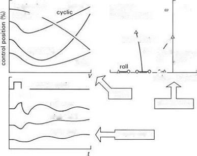
The sketches in Fig. 2.17 illustrate typical ways in which trim, stability and re­sponse results are presented; the key variable in the trim and stability sketches is the helicopter’s forward speed. The trim control positions are shown with their character­istic shapes; the stability characteristics are shown as loci of eigenvalues plotted on the complex plane; the short-term responses to step inputs, or the step responses, are shown as a function of time. This form of presentation will be revisited later on this Tour and in later chapters.

The reader of this Tour may feel too quickly plunged into abstraction with the above equations and their descriptions; the intention is to give some exposure to math­ematical concepts which are part of the toolkit of the flight dynamicist. Fluency in the

lateral
longitudinal cyclic””-”^	о hover a high speed
rad/s

short! period /

spiral ft (1/s)

STABILITY

pitch rate

FIFSPQNSE

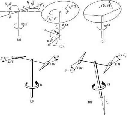
Fig. 2.18 f rotor flapping and pitch: (a) rotor flapping in vacuum; (b) gyroscopic moments in vacuum; (c) rotor coning in air; (d) before shaft tilt; (e) after shaft tilt showing effective cyclic path

parlance of this mathematics is essential for the serious practitioner. Perhaps even more essential is a thorough understanding of the fundamentals of rotor flapping behaviour, which is the next stop on this Tour; here we shall need to rely extensively on theoretical analysis. A full derivation of the results will be given later in Chapters 3, 4 and 5.