Flows in the Vicinity of Edges

In region De, i. e., in the vicinity of the edges of the wing (/1 and I2) and the wake Z3, one has to derive local asymptotic descriptions of the flow.

Inspection of the Laplace equation shows that for sufficiently large radii of curvature of planform contours (pe h0), the flow near the edge can be

considered two-dimensional in the plane normal to the planform contour. This circumstance considerably facilitates the analysis of edge flows. In particular, effective methods of the functions of the complex variable can be used to account either for the specifics of the geometry of the edge (thin or thick, with endplates, etc.) or for the physics of the local flow (shock or shock-free entry at the leading edge, vortex roll-up at wing’s tips, jet and rotating flaps, etc.). Examples of various edge flows are shown in Fig. 2.3.

Here one considers an example of a sharp edge with a small vertex angle. Later on, when examining particular effects, such as the jet blowing from the trailing edge or the use of rotating flaps, one will have to consider corresponding local flows.

" G

Fig. 2.3. Possible local flows in the problem of a wing in the extreme ground effect.

Consider a flow near the leading edge l. Introduce a local coordinate system vOy, where v is an external normal to the planform contour, and stretch independent variables

v = v/K, y = y/K> (2-34)

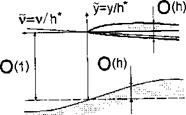
where /1* = hl(l, t) is an instantaneous relative distance of the edge vertex from its projection upon the ground. Parameter Z, as introduced previously, represents the arc coordinate measured along the planform contour. Note that due to assumption (2.1) both the wing and wake surfaces have spanwise and chordwise slopes of the order of О(h0). Therefore, the edge flow problem formulation can be linearized. In fact, as prescribed by (2.1), in the stretched local region De the distances of points on the wing’s upper and lower surfaces from the horizontal line у = 1, as well as the distances of points of the ground surface from horizontal line у = 0 are of the order of О(h0) (see Fig. 2.4). Therefrom with an asymptotic error of the order of О (ft^), the tangency conditions on the wing and on the ground can be transferred to horizontal lines у — 0 and у — 1, respectively.

The corresponding problem for the leading (side) edge flow velocity po­tential (pe = (fe can be formulated as follows:

d2<fe d2<pie dy2 dv2	= 0, (у, і>) Є Д.;	(2.35)
dVe.2 , dy ~ h°dg’	|i>| < oo, у = 0 + 0;	(2.36)
9<Ple u2 A dy ~ h°du’	v < 0, у = 1 + 0;	(2.37)
d<Pe,2 . ay =	o’ 1 r-H II *5» О VI	(2.38)

Parameters gZu, gZi, and dg depend on arc coordinate Z and time t and have to be determined in the process of matching with the asymptotic solutions constructed in the upper and channel flow regions. Note that without loss

Fig. 2.4. Local flow in the vicinity of the edge with a finite vertex angle.

of generality, it is possible to set dg = 0. In the problem for the flow near a leading edge, the boundary conditions at infinity on the wake and at the trailing edge have been lost. Their influence on the leading edge flow will be recovered by matching with the asymptotic descriptions of the velocity potential in the channel and upper flow regions.

Due to the linearity of the local problem, its general solution can be presented in the form

<fle = Gl^o^ae + + 0*3 + &4^о? (2.39)

where di are parameters to be determined through matching. Function </?ae is a homogeneous solution, satisfying the condition of no normal velocity on the wing and ground surfaces (du = d = dg = 0). This homogeneous solution corresponds to a circulatory flow around the edge. Function (ръе represents a nonhomogeneous solution, which is generated by a prescribed normal velocity upon the wing and the ground. Both </?ae and <РЬе are of the order of 0(1). Linear combination a^hQv + <24 automatically satisfies the Laplace equation and does not violate the flow tangency condition on solid boundaries.

We turn to determination of functions <pae and <рье- To find solution of the homogeneous problem for the flow past the leading (side) edge, we perform a conformal mapping of the local flow domain De onto the upper half plane

= 77 > 0 of the auxiliary complex plane ( = £ + і r) by the Christoffel – Schwartz integral; see Lavrent’ev and Shabat [129]. The correspondence of points in the physical plane (i = v + і у and auxiliary plane ( is illustrated in Fig. 2.5.

The mapping function has the form

li = — (1 + C + lnC)> (2.40)

7Г

where і = д/—Ї is an imaginary unit. For purely circulatory flow around the edge in the plane of the complex potential /ae = <£ae + i^ae, the flow with unit velocity at the left infinity v = – 00 is represented by a strip of unit width. Conformal mapping of this strip onto the upper half plane > 0 is realized by the function

/ae = ^ae "b І Фа-е ~ in £. (2.41)

7Г

Eventually, the solution of the homogeneous problem is given by the formulas (2.40) and (2.41). Excluding the auxiliary variable £, we obtain the following relationship between the “physical” complex plane Д = z/+i у and the complex potential /ae = </?ae + і Фае, representing the homogeneous component of the problem solution.

тгД = 1 + ехр(тг/ае) + тг/ае. (2.42)

The flow pattern, corresponding to the homogeneous solution (pae is depicted schematically in Fig. 2.6. At points on the wing surface near the leading (side) edge, where Де = v? ae + і, /і = v + i, v < 0, the potential (pae can be determined through the following implicit relationship:

ТГй = 1- ЄХр(7Г(/?ае) + ТГ^ае-

It can be shown that the flow velocity has a standard square root singularity at the leading edge. In fact, in the immediate vicinity of the edge vertex v —> 0 — 0, (pae —> 0, and it follows from the expansion of equation (2.43) that

I 1

TTP~ 1 – (1 + TT^ae + ^Vae + ‘ ‘ ‘) + ^ae ^ (2‘44)

wherefrom for и —у 0 — 0,

ss0′ (245)

To match the flow potentials in regions Du and D, one needs the asymp­totic representations of the edge flow potential (pae far from the edge. Turning to the variable v = h*ei> = h0h*ev and setting h0 to zero for fixed v — 0(1), one obtains

7Г1У h0h*f

• on the upper surface of the wing (v — v/h*e —> — oo, у — 1 + 0),

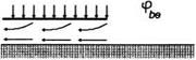Fig. 2.6. Flow patterns corresponding to the homogeneous (fae and nonhomogeneous <ръе components of the edge flow potential.

(2.47)

• on the lower surface of the wing (y = v/h*e —>■ — oo, у = 1 — 0)

We turn to the determination of the nonhomogeneous solution </?be – Using the same mapping function (2.41), one comes to the following problem for a complex conjugate velocity Wbe = ^be — i^be in the auxiliary plane £: Find an analytic function u>be(C) in the upper half plane = r] > 0 in terms of its imaginary part Эгиье — —^be given on the axis £ (see Fig. 2.7).

It can be verified that the following expression satisfies the problem under consideration:

Wbe = – [(du – di)ln(l + C) + d In £]. (2.48)

7Г

At points on the wing in the vicinity of the edge (£ = £ < 0),

ube = SRu>be = l[(du — di) In |1 + ^| + diln|^|]. (2.49)

7Г

The velocity potential corresponding to the nonhomogeneous solution can be derived by means by integrating(2.49):

^be = Uhedv. (2.50)

Jo

At points on the wing surface, the auxiliary variable £ = Щ is related to the variable v in the following way:

тгі/ = 1 + £ + 1п|£|, £ < 0. (2.51)

The flow pattern corresponding to a nonhomogeneous solution is presented schematically in Fig. 2.6. In the particular case of an infinitely thin edge (zero vertex angle du = d — d 3), the following expression for (ръе can be derived from the previous more general relationships:

• on the upper surface of the wing (v — v/h*e —» — oo, —oo)

To match the edge flow potential with the velocity potentials in regions Du and D, we need to know asymptotic representations of ще and c^be far from the leading (side) edge. These can be found in the form

• on the lower surface of the wing (v —» —oo, у = 1 — 0, £ —0 — 0)

—У 7Г/10Л*Є/

(2.55)

Taking into account expressions (2.39) and (2.45) we obtain the following estimate of the behavior of the velocity near the leading edge of the lifting surface along the normal to the planform contour:

where the “minus” sign corresponds to the upper surface of the wing, and the “plus” sign corresponds to the lower surface of the wing. Formula (2.57) is useful for calculating the suction force at the leading edge of the lifting system in both steady and unsteady motion.

Note that the asymptotic solution of the problem for the flow near the edge of a vortex sheet in the extreme ground effect has the same structure as that for an infinitely thin leading (side) edge.

Near the trailing edge /2, the velocity potential ipe = ipte should sat­isfy not only the flow tangency conditions on the wing and the ground but also comply with the dynamic and kinematic conditions on the vortex sheet emanating from the wing due to unsteady and three-dimensional effects. Ex­cluding the homogeneous component of expression (2.39) which incorporates a square root singularity for the flow velocity at the edge, we can write the velocity potential ipte for the flow in the vicinity of the trailing edge in the form

<Pte = Mo^be + b2hlv + b3h0,

where v = v/h*(l, t) = vjh^ and y>be is given by the formula

(Phe= Ще dP, (2.59)

Jo

Ще = ^[(eu – ei) In |1 + f | + e In |£|]. (2.60)

The auxiliary variable £ is related to v by equation (2.51). Parameters eu, e and bi, 62, bs are unknown and have to be determined by asymptotic match­ing. It is essential to note that parameters 62 and 63 have different magnitudes on the upper (y = y/h*e = 1 + 0) and lower (y = y/h*e = 1—0) surfaces of the vortex sheet behind the trailing edge, i. e., Ф b^ and 63 ф b% . This is caused by the jump discontinuity of the velocity potential and the tangential velocity at the trailing edge I2, the latter in the case of unsteady flow. At the same time, the solution satisfies the condition of the continuity of the normal velocity component across the vortex sheet. In the particular case of an infinitely thin trailing edge (zero vertex angle eu = e = e), it follows from (2.59) and (2.60) that

є 1

<РЪе = ~ ^(тг^ае – 1) – o^ae]- (2-61)

7Г Z

The asymptotic representation of иъе and сръе far from the trailing edge can be found from expressions (2.53)-(2.56) by replacing duд by еид and h*e by h*e. Note that the solutions of local flow problems, presented above, lose validity in the vicinity of the order of О(h0) of the corner points of con­tours 11,^2, where the flow is essentially three-dimensional. Near such corner points, additional solutions should be constructed, but this question will not be discussed here.