. NONLINEAR ANALYSIS IN THE FACE OF PARAMETRIC UNCERTAINTIES
As an other example, consider the closed loop system of Figure 7.2. Ф represents a nonlinearity, whereas the LFT Fi(P(s), Д2) represents a
parametrically uncertain transfer matrix, i. e. N2 is a real model perturbation.
The Sinusoidal Input Describing Function (SIDF) N(X, w) is introduced for the nonlinearity 2> . For the sake of simplicity, N (N, N ) is defined for a SISO nonlinearity. The definition is however readily extendible to the general case of a MIMO nonlinearity. A sinusoidal input u(t) = Xsin(u>t) is applied to Ф. The output of Ф, which is supposed to have odd symmetry, is written as:
y(t) — Rsin(wt) + Scos{wt) + e(t) (7.5)
where contains the super harmonic part of signal y(t). The SIDF is the complex gain:
N(X, w) = (7.6)
 |
In the context of the first harmonic approximation, the signal e(t) is assumed to be filtered by the low-pass transfer matrix Fi(P(s),A2).
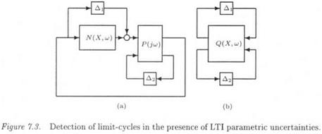
The MIMO nonlinearity N is now replaced by N(X,2) + Ді in the closed loop system of Figure 7.2 (see Figure 7.3.a). Roughly speaking, Ді is a block of neglected dynamics, which takes into account the super harmonic part e(t) of the signal y{t) (Katebi and Zhang, 1995; Ferreres and Fromion, 1998). N 1 is only known by the relation:
![]() <т(Д) < а(Х, ш)
<т(Д) < а(Х, ш)
where n)N) n) is a known function of the magnitude X and frequency w of the limit-cycle.
Figure 7.3.a is then reshaped into Figure 7.3.b. A sufficient condition for the absence of limit-cycles in the nonlinear closed loop is given by:
a(Fl(Q(X, w),A2)) < —(7.8)
a(X, u))
As in the previous section, for given values of X and w, the problem consequently reduces to the issue of checking a small gain condition in the presence of a real model perturbation Д2: The aim is indeed to compute the maximal amount of parametric uncertainties, for which the sufficient condition (7.8) for the absence of limit-cycles remains satisfied.


