
Our heavyweight helicopter equal in the world does not have
In Rostov started production of the most load-lifting rotary-wing car The Russian holding «Helicopt[...]

Everything about aircrafts and helicopters. News and events in aviation worldwide. Civil, transportation, military helicopters and airplanes.

Everything about aircrafts and helicopters. News and events in aviation worldwide. Civil, transportation, military helicopters and airplanes.

Everything about aircrafts and helicopters. News and events in aviation worldwide. Civil, transportation, military helicopters and airplanes.

Everything about aircrafts and helicopters. News and events in aviation worldwide. Civil, transportation, military helicopters and airplanes.


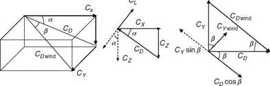
At times, it is useful to work with equations expressed in polar coordinates for the following reasons:
• It is more convenient to use equations in polar coordinate terms as the aerodynamic forces and moments are easier to visualize and express in terms of angle of attack a, sideslip angle b, and velocity V.
• Flow angles a and b can be directly measured, and hence yield simple observation equations.
• Primary disadvantage, however, is that the system becomes singular at zero velocity, for the hover condition of a rotorcraft. Also, singularity occurs at beta equal to 90°.
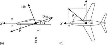
V, a, and b in terms of u, v, and w are given by the following expressions (Figure 3.11):
![]() _1 w a = tan — u
_1 w a = tan — u
b = sin-1 V
Differentiating the above equations, we get
![]()
|
|
|
|
|
|
|
|
|
|
|
|
|
![]()
|
|||
|
|
||
|
|||
|
|||
|
|||
|
|||
|
|||
|
|||
|
|||
|
|||
Any of the above forms (rectangular or polar) can be used to describe the aircraft motion in flight. Note that there are no small angle approximations used, but equations have singularity at U = 90°. Further, there are several trigonometric and kinematic nonlinearities in the 6DOF equations.
Analysis of the full 6DOF equations would require a nonlinear program. The 6DOF model postulate is useful where nonlinear effects are important and coupling between the longitudinal and lateral modes is strong.
Although it is possible to analyze the 6DOF models, it is always a good idea to work with simplified models. These will be discussed in Chapter 5.
 Без верификации!")