. Linearization in general

The assumptions made to establish the above approximate results have not been dis­cussed; we have neglected detailed blade aerodynamic and deformation effects and we have assumed the rotorspeed to be constant; these are important effects that will need to be considered later in Chapter 3, but would have detracted from the main points we have tried to establish in the foregoing analysis. One of these is the concept of the motion derivative, or partial change in the rotor forces and moments with rotor motion. If the rotor were an entirely linear system, then the total force and moment could be formulated as the sum of individual effects each written as a derivative times a motion.

This approach, which will normally be valid for small enough motion, has been established in both fixed – and rotary-wing flight dynamics since the early days of flying (Ref. 2.13) and enables the stability characteristics of an aircraft to be determined. The assumption is made that the aerodynamic forces and moments can be expressed as a multi-dimensional analytic function of the motion of the aircraft about the trim condition; hence the rolling moment, for example, can be written as

+ terms due to higher motion derivatives (e. g., p) and controls

For small motions, the linear terms will normally dominate and the approximation can be written in the form

L — Ltrim + Luu + Lvv + Lww + Lpp + Lqq + Lrr

+ acceleration and control terms (2.46)

In this 6 DoF approximation, each component of the helicopter will contribute to each derivative; hence, for example, there will be an Xu and an Np for the rotor, fuselage, empennage and even the tail rotor, although many of these components, while dominating some derivatives, will have a negligible contribution to others. Dynamic
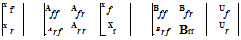
effects beyond the motion in the six rigid-body DoFs will be folded into the latter in quasi-steady form, e. g., rotor, air mass dynamics and engine/transmission. For example, if the rotor DoFs were represented by the vector xr and the fuselage by xr, then the linearized, coupled equations can be written in the form

(2.47)

We have included, for completeness, fuselage and rotor controls. Folding the rotor DoFs into the fuselage as quasi-steady motions will be valid if the characteristic frequencies of the two elements are widely separate and the resultant approximation for the fuselage motion can then be written as

xf — ^Aff — AfrArr Af j xf = — AfrA-r Bf] uf + [Bfr — AfrA— Brr] Ur

(2.48)

In the above, we have employed the weakly coupled approximation theory of Milne (Ref. 2.14), an approach used extensively in Chapters 4 and 5. The technique will serve us well in reducing and hence isolating the dynamics to single DoFs in some cases, hence maximizing the potential physical insight gained from such analysis. The real strength in linearization comes from the ability to derive stability properties of the dynamic motions.