Stability Diagram

It is easily seen from Eq. (3.16) that the relationship between rnAt and rnAt is not one to one. This means that there are spurious numerical solutions. These spurious solutions could cause numerical instability, so it is necessary to find out about their characteristics.

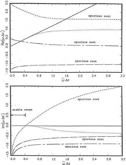
Figure 3.1. The real and imaginary parts of the four roots of « At as functions of «At.

Eq. (3.16) may be rewritten in the form as follows:

^ ^ + V2 + (b0 + =At)z – = 0. (3.20)

where z = elmAt. Thus, given a «At, there are four roots of elmA. In other words, there are four values of «At that would give the same «At when substituted into Eq. (3.16). For the values of bj (j = 0, 1, 2, 3) given by formula (3.19), the val­ues of the four roots of «At as functions of «At have been found. The real and imaginary part of these roots over the range 0 < «At < n are plotted in Fig­ure 3.1. In the range «At < 0.41, the imaginary parts of all the four roots are neg­ative. Recall that the solution «, given by the inverse transform of Eq. (3.11), is a superposition of elemental solutions having time dependence of the form e-lmt. If Im(«) is negative, the solution is damped in time. However, for «At > 0.41,

Figure 3.2. Region of stability in the complex mAt plane.

one spurious root has a positive imaginary part. The solution corresponding to this root will grow, in time overwhelming the physical solution, and lead to numerical instability.

On examining the real parts of the four roots, it is seen that one of the roots gives mAt = mAt over the range mAt < 0.41. This is the physical root. The others are spurious. The physical root has a very small imaginary part up to mAt = 0.41. That is, there is very little numerical damping. A more detailed investigation reveals that, for this root, Im (mAt) = -0.118 x 10-4 for mAt = 0.19. This is reasonably small. It is recommended that At be chosen such that mAt < 0.19. This would automatically guarantee numerical stability and negligible numerical damping.

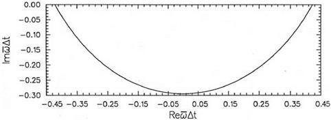
In most wave propagation problems, to be discussed later, mAt is real. In this case, this stability consideration is sufficient. However, if the wave is damped by some physical process, or artificial damping is added to the computation scheme for the purpose of removing spurious waves from the numerical solution, then mAt is complex. To include this more general case, it is necessary to consider the four solutions of Eq. (3.20) for mAt in the complex plane. It is straightforward to find that the stable region (all the four roots of mAt have a negative imaginary part) is confined to a small nearly semicircular region in the lower mAt plane. This is shown in Figure 3.2. This stability diagram plays an important role in the choice of time step At in time marching computation. Numerical stability will be discussed in Chapter 5.

EXERCISES 3.1. Construct an optimized two-level time marching scheme for the differential equation

F (u).

Find the stability region in the complex mAt plane. 3.2. Consider the solution of the initial value problem

d U	д U	(A)
~dt	+ c – = 0 д X
	– = e-(ln2)( 5AX)2	(B)

by finite difference approximation. Let the spatial derivative be approximated by a second-order central difference equation. The convective wave equation becomes

dul c

~dt _- 2^(Ul+1 – Ul-1 X

where l is the spatial index. Difference-differential equation (C) may be integrated by the four-level optimized time marching scheme. On writing out in full, the finite difference equations are

E(n) _ C (,/n) U(n) ) _ 2AxUl+1 Ui-1′	(D)
3 uln+1) _ u(n + AtY^bjEtj). j_0	(E)

Consider a Fourier-Laplace transform component of the solution

U^n’) __ Ае^(1аДх— n^At)

Perform a Von Neumann stability analysis of the finite difference scheme by sub­stituting Eq. (F) into (D) and (E). Show that this yields the dispersion relation as follows:

ш(ш) _ ca(a),

where a is the stencil wave number of the second-order central difference scheme and ш is the angular frequency of the four-level time marching scheme.

(a) Show that the scheme is stable if

0. 41 Дх

At <————

c

(b) Implement the time marching scheme on a computer. Take At to be slightly larger than that given by Eq. (H). Compute the solution in time up to t _ 400 with (B) as the initial condition to see whether the solution is unstable (i. e., grows exponentially in time).

(c) Verify computationally that, if At is chosen according to condition (H), the numerical scheme is stable. Furthermore, if At is taken to be less than or equal to 0.19 Дх/c, an excellent numerical solution can be obtained.