Very Thin Profiles (Skeleton Theory)

Fundamentals of skeleton theory As was stated above, the very thin profile (skeleton profile) is obtained by superposition of a translational flow with that of a distribution of plane potential vortices. This theory has therefore been termed the theory of the lifting vortex sheet. It was first developed by Birnbaum and Ackermann [8] and by Glauert [17], and later expanded in several treatises, particularly by Helmbold and Keune [22, 32], Allen [3], and Riegels [49].

For the following discussion a coordinate system as shown in Fig. 2-20a is used. Accordingly, the profile chord coincides with the x axis. The coordinate system origin lies on the profile leading edge. The mean camber line is given by z^{x). From Fig. 2-20a, the mean camber line is seen to be covered with a continuous vortex distribution. With the assumption that the skeleton profile has only a slight camber and, therefore, rises only a little above the profile chord (x axis), the vortex distribution can be arranged on the chord instead of the mean camber line (Fig.

2- 20b). The mathematical treatment of the problem is considerably simplified in this way.

The vortex strength of a strip of width dx of the vortex sheet is, from Fig.

2- 20 b,

Неге, к is the vortex density (vortex strength per unit length) or the circulation distribution. By applying the law of Biot-Savart, the velocity components in the x and z directions, respectively, that are induced by the vortex distribution at station x, z are

C “t[7]’2)- 2* (х-*)> + г‘ ІХ’ 0 (245a) C 10 {x, *) — 2jr jk (X ) ^ _J_ г2 dx (245b) О

For slightly cambered profiles, the velocity components on the skeleton line are approximately equal to the values on the profile chord (z = 0). The velocity components on the chord are obtained through limit operations as z -> 0 of Eqs. (245a) and (2456)

were introduced in Sec. 2-1, with c being the chord length.

The velocity component и is proportional to the vortex density. The upper sign is valid for the profile upper surface, the lower sign for the lower surface. When crossing the vortex sheet, the velocity component и changes abruptly by an amount

Au — uu—Ui — k (248)

The integral for the velocity component w has a singularity at X’ = X*

The distribution of the vortex density on the chord is determined by the kinematic flow condition, which requires that the skeleton line is a streamline. Specifically, a translational velocity Ux is superimposed on the vortex distribution that forms the angle of attack a with the chord (Fig. 2-20).

The kinematic flow condition can also be formulated by the requirement that the velocity components normal to the mean camber line must disappear. Within the framework of the above approximation, it is sufficient to satisfy this condition on the chord instead of the mean camber line, resulting in

	(249)

This equation relates the angle of attack a and the ordinates of the camber to the induced normal velocities w.

The velocity distribution on the profile surface and the vortex density are related by

U(X)=U„ + u(X)**U„±lk(X) (2-50)

This relationship is valid for small angles of attack according to Eq. (246a).

The Kutta condition, Sec. 2-2-2, requires that the velocities on the profile upper and lower surfaces be equal at the trailing edge. It is required, therefore, that in Eq. (2-50),

k = 0 for X = 1 (2-51)

The total circulation around the profile is determined from the distribution of the vortex density as

Г= Jk(x) dx = c j’lc(X)dX

The pressure difference between the lower and upper surface is obtained by means of the Bernoulli equation:

Pi Pu Q Ifoo А Ы Q Uook

With Eq. (248), the dimensionless pressure coefficient takes the form

with q„ —qUlell being the dynamic pressure of the incident flow. Consequently, the distribution of the vortex density produces directly the load distribution over the profile chord. From Eq. (2-10), the lift coefficient = L/q„bc is expressed by

cL = / AcJX) dX

The latter relationship may also be found from the interrelation of lift and circulation after the Kutta-Joukowsky equation (2-15) for wTC = Ux. Equation (2-12) yields the pitching-moment coefficient relative to the profile leading edge, cM =M/qoabc1 (tail-heavy = positive):

(2-55 b)

0

Computation of the mean camber line from the distribution of circulation Deter­mining the shape of the mean camber line and the angle of attack from a given distribution of circulation k(X) requires two steps. First, from Eq. (246b), the distribution of the induced downwash velocity w(X) is obtained along the profile chord. Then, this distribution is introduced into the kinematic flow condition, Eq. (249), and the following expression for the shape of the mean camber line is obtained by integration over X:

These two steps may be combined into one equation by introducing Eq. (246b) into Eq. (2-56) and integrating over X. The angle of attack and the integration constant C are determined in such a way that the ordinates of the mean camber line disappear on the leading and trailing edges, resulting in

for the mean camber line and

(2-58)

for the angle of attack as measured from the chord.

In the case of a constant distribution of circulation along the profile chord, к — 2U«,C, Eqs. (2-57) and (2-58) yield, for the mean camber line and the angle of attack,

— ■. ZM(X) = – — [(1 – X) ln(l – X) + X lnX] with Л = 0 (2-59)

The maximum camber height is h/c = (In 2jn)C = 0.221C and lies at 50% chord. This mean camber line is found in NACA profiles of the 6-series (see Fig. 2-2c; a = 1.0). The lift coefficient is obtained from Eq. (2-54b) as

Following up on the investigations of Birnbaum and Ackermann, Glauert [17] proposed the following Fourier series expansion for the circulation distribution in the two-dimensional airfoil problem:

(2-61)

X = 1(1 – j – cos 9?)

so that on the leading edge X = 0 and = u, and on the trailing edge X = 1 and V? = 0. Each term in Eq. (2-61) satisfies the Kutta condition, Eq. (2-51).

By introducing the expression for the distribution of circulation, Eq. (2-61), into the equation for the induced downwash velocity, Eq. (2-46b), the simple relationship*

(2-63)

is found after integration.

The interrelation of the Fourier coefficients of Eq. (2-63), the shape of the mean camber line, and the angle of attack are obtained with the help of Eq. (249) as

With a given distribution of the circulation, this is a differential equation for the mean camber line Z^SX).

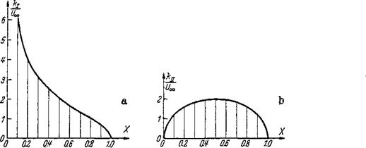
The first two terms in Eq. (2-61) represent particularly simple mean camber lines: The distribution of circulation of the first standard distribution becomes

The distribution к is shown in Fig. 2-21 a. The induced downwash velocity is determined from Eq. (2-63) to be wlU„ = —A0, leading to

Further, from the kinematic flow condition, Eq. (2-64), it follows that the profile inclination dZ^/dX must be constant. This is possible only when Z^ = 0, and, therefore,

(2-66)

It has thus been shown that the first normal distribution represents flow about the inclined flat plate.

The second normal distribution is given by

1c — A1 k[j = 2 Uco Аг sin= 4£/co Ах |/Х(І —X) (2-67)

/

Figure 2-21 The first and the second normal distributions; circulation distribution by Eq. (2-61). (a) The inclined flat plate. (b) The parabolic skeleton at zero angle of incidence.

This is an elliptic distribution (Fig. 2-21 b). The induced downwash velocity is obtained from Eq. (2-63) as

^ = — cos cp = — (2 2Г – 1)

C/oo

and with Eq. (2-56), the shape of the mean camber line is given by

zW=AtX(l – X) = 4jX(l – X) with a = 0 (2-68)

This is a parabolic mean camber line with camber height h/c = Ai/A0. The results obtained for the inclined flat plate and the parabolic camber without angle of attack agree with the exact solutions found by the method of conformal mapping for small angles of attack, Secs. 2-3-2 and 2-3-3, respectively.* In particular, the relationships for lift and pitching-moment coefficients are also valid.

Computation of the aerodynamic coefficients Equations will now be presented that allow one to compute the aerodynamic coefficients directly from a given mean camber line. The lift coefficient is obtained from Eq. (2-54Z?) after integration t with the help of Eqs. (2-61) and (2-62) for the distribution of circulation as

cL=7t(2A0+Al) (2-69)

In the same way, the pitching-moment coefficient relative to the leading edge is obtained from Eq. (2-55b) as

Cm — —^"(2-d. o 2A^ – j – A%) (2-70)

This equation was first presented by Munk [41].

*Note that %Sc — X — .

tin this process, most of the integrals over <p disappear as a result of the orthogonality conditions of the trigonometric functions.

The angle of attack for zero lift (cL =0) is obtained by setting 2A0 = —A1} and the zero-lift moment coefficient becomes cM0 =—(ir/4)(Ai+A2). Conse­quently, the pitching-moment coefficient can also be written as

1

CM – CMO

From Eq. (1-29), the neutral-point location is given by —dcM/dcL = xNjc. Consequently, the distance of the neutral point from the leading edge becomes

XN _ 1

c 4

which is independent of the shape of the mean camber line.

The Fourier coefficients are found through Fourier analysis:

71 n

1 Г dZ{s) 9 Г dZ{s)

A0=cx-—J ~jY~d(P An=-^J -jj-costt <pd(p (n> 1) (2-73)

о 0

The integrals can be transformed through integration by parts into terms in which the camber line coordinates replace the camber line inclination dZ^/dX. By introducing the coefficients A0 and Ax into Eq. (2-69), the relation

dcT

it=2* w

is obtained for the lift slope, independent of the camber line shape, and the lift coefficient from Eq. (1 -23) is

cl~ 2іт(а—а0) (2-75)

The equations for a0 and cM0 are given in Table 2-1.

On the profile leading edge, X = 0, that is, = nr, in general the vortex density and consequently the velocity are infinitely large (Eq. 2-61). There is an angle of attack, however, for which the velocity remains finite on the leading edge. In Sec. 2-3-3, the designation of angle of smooth leading-edge flow was introduced for this angle of attack. This angle as can be determined from Eq. (2-61) by setting A0 = 0. The expressions for as and for the lift coefficient for smooth leading-edge flow are also presented in Table 2-1.

If there is flow around the leading edge, the velocity is infinitely high, streaming either from below to above, or vice versa. The strong underpressures near the leading edge produce a force acting upstream on the leading edge, called suction force in Sec. 2-3-2. The suction force coefficient cs = S/q„bc can be expressed by

1

cs = – j!- f k{X) w(X) dX

V CO J

0

Introducing Eqs. (2-61) and (2-63) into this equation yields

c, s = 2 я A‘i

Table 2-1 Compilation of formulas for the aerodynamic coefficients of cambered profiles of finite thickness Lift slope dcL da l 2 f Z 2n 1 -|—— ———— dm 1 71 J Sin^) r j 2л(і + 2 ez^ Zero-lift angle «0 n 2 Г Zw n J 1 — cos <p (^ 0 N -1 2 E вт z<s> Neutral-point location •Lv c 1 / 2 Г 1 + 2008^- 2003 2, * 4 1 71 J Sill Cp T J t (і + Ц’с-z’,::) Zero moment см о f 2cos,>-cos2,, J 1 — cos q> 0 2 E D, n Z<’> " Hi Angle of incidence for smooth leading-edge flow as 71 2 Г cos m ч, / . „ Zl>)dtp n J sm^ T 0 N -1 2 І7 Z<*> ^ и* 4» Lift coefficient for smooth leading-edge flow CLS n r ZM 4 . 0 dtp J sin – (p T 0 JV-l 2 27 Z(-> иг /ti ‘ See correction in [50].

and with Ci of Eq. (2-69) and cLS =nA1,

cs = 2^(cl ~cls)2 (2-77)

Consequently, the suction force is zero for smooth leading-edge flow, but grows with the square of (cL — cLS).

For a given distribution of circulation k{X), the coefficient A0 in Eq. (2-61) is obtained by the limit operation

A0 = lim [kQOVX]

ZUac 0

In the integral formulas of Table 2-1 for the computation of the various coefficients, only the. distribution of the mean camber coordinates appear

besides certain trigonometric functions of ip. In addition, simple quadrature formulas are given for the numerical evaluation of the integrals. Accordingly, the profile coordinates Zm = Z(Xm), at the stations Xm are multiplied with once-for-all-computed coefficients, Fm, and the sums are then formed of these products (see

Table 2-2).

In Table 2-3 a few results are presented that can easily be verified. Case (a) refers to a uniformly cambered skeleton line from Eq. (2-6); case (b) refers to an asymmetrically cambered line from Eq. (2-5).

For the case of a simple parabolic mean camber (Xh = |), the numerical values are

ot0=-2^ cM0 = -7tj as = 0 cls=4ttj (2-78)

u L C-

The profiles with fixed aerodynamic centers according to the discussion in Sec.

1- 3-2 are obtained from the above skeleton family by setting смо = 0. From Table

2- 3, case (b), it follows immediately that b = — f. This camber line has an inflection point (S shape). The case b = 0 is again the simple parabola skeleton.

Table 2-2 Coefficients А, В, C, D, E, F for the computation of the aerodynamic coefficients of Table 2-1 forrV= 12 (after Riegels (49,50]) m Хщ Am Вщ с Вщ F 1 т 1 0.9830 0.6440 -4.8919 0.6864 -7.9370 -2.4032 15.6333 2 0.9330 0 0 0.1667 -0.2267 0 0 3 0.8536 0.2357 -0.5690 0.3333 -1.0790 -0.2357 2.0944 4 0.7500 0 0 0.2887 -0.1309 0 0 5 0.6294 0.1726 — 0.2249 0.2387 -0.4210 -0.0462 1.1224 a 0.5000 0 0 0.3333 0 0 0 r- І 0.3706 0.1726 -0.1324 0.0601 -0.1402 0.0462 1.1224 8 0.2500 0 0 0.2887 0.1309 0 0 9 0.1465 0.2357 -0.0976 -0.3333 0.0318 0.2357 2.0944 10 0.0670 0 0 0.1667 0.2267 0 0 11 0.0170 0.6439 — 0.0848 -1.8017 0.1197 2.4032 15.6333

Table 2-3 Aerodynamic coefficients of uniformly and asymmetrically cambered skeleton lines Coefficient (a) Skeleton from Eq. (2-6) (b) Skeleton from Eq. (2-5) Zero-lift angle a° h 1 c 1-Xh – | (4 + 3b) Zero-moment coefficient cMo n h xh0 – 2Xh) 2 c 1-Xh – ^*(8 + lb) Angle of incidence for S. L.E. F.* as 1 h 1 —2Xh 2 c xha-xh) 1 OO | b – El Lift coefficient for S. L.E. F.* CLS h 1 77 c xha – xh) a(2 + b) *Smooth leading-edge flow.

In the NACA systematic listing, various skeleton line shapes are used (see Sec.

2- 1).

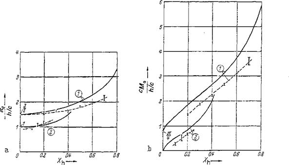
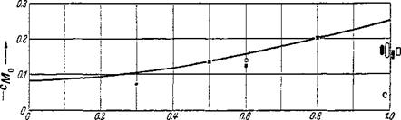
Four-digit NACA profiles In Fig. 2-22, zero-lift angles of attack and zero moments are plotted versus the maximum camber height (crest) location. Test results [1] are also shown for comparison with theory. Because of the slight effect of profile thickness in the range of thickness ratios 0.06 < t/c < 0.15, a mean curve of experimental data is shown. The plotted bars represent three data points each for cambers h/c = 0.02, 0.04, and 0.06. The agreement of theory and experiment is

Figure 2-22 Zero-lift angle of attack a0 and zero-moment coefficient cjvf0 of NACA skeleton lines. Comparison of theory and experiment from NACA Repts. 460, 537, and 610. Curve 1, four-digit skeleton lines. Curve 2, five-digit skeleton lines.

satisfactory. As a result of friction, the deviations increase somewhat with a downstream shift of the camber crest.

Five-digit NACA profiles In Fig. 2-22, results for zero-lift angle and zero moment are presented for the skeleton lines without inflection points. Test results from [1] are also shown. The influence of the profile thickness is again negligibly small. The plotted test data are the results for values of c^s ~ 03, 0.45, 0.6, and 0.9. Agreement between theory and experiment is better than in the case of the four-digit NACA profiles.

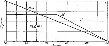
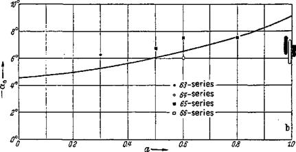
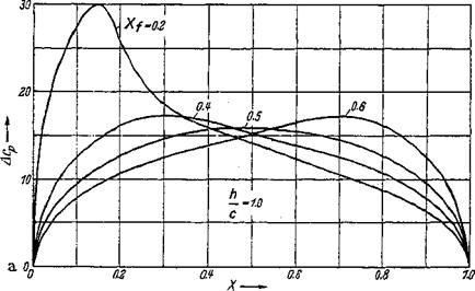
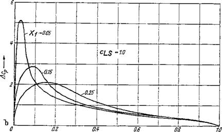
NACA 6-profiles The skeleton lines of the NACA 6-series have been established from purely aerodynamic considerations. Preestablished are the resultants of the pressure distributions on the lower and on the upper profile surfaces (Fig. 2-23a). The corresponding skeleton lines are presented in Fig. 2-2c.

For the aerodynamic coefficients, the following expressions are established:

(2-796)

(2-79 c)

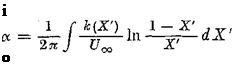
Zero-lift angles of attack and zero-moment coefficients for cLS = 1 are given in Fig. 2-23b and c versus the quantity a. These results are compared with test results of NACA Rept. 824 and show satisfactory agreement.

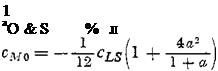
Bent plate (flap, wing, control surface) Another valuable application of the skeleton theory is found in the calculation of the aerodynamic coefficients of the flap wing. By replacing the flap wing by a skeleton line, the bent plate, Fig. 2-24, is obtained. This problem was attacked first by Glauert [18].

With the assumption of a small deflection angle r]f, the ordinates of the skeleton line ZW = Zf, relative to an imaginary chord connecting the leading edge with the trailing edge of the deflected flap, are

zf=Wvf

where f— Cf/c is the flap chord ratio (see Sec. 3-1-1).

Since the profile inclinations are constant within the ranges of Eq. (2-80), integrations for the determination of aerodynamic coefficients can easily be performed. It is expedient to introduce in addition the following relationship for the position of the station:

The change of the zero-lift angle with flap deflection is measured relative to the fixed portion of the profile (wing, stabilizer) rather than relative to the imaginary chord. The change of angle of attack (= change of the zero-lift angle with flap deflection) is then given by

= ~ ~ (sin Pf + Pf) = ~~ ~ (%А/0 ~ V) arcs^ri VV ) (2-82a)

a—— Figure 2-23 Aerodynamic coefficients for skeleton lines of the NACA 6-profiles at the lift coefficient of the smooth leading-edge flow Cjr^ =1.0. Comparison of theory [Eqs. (2-79a)~ (2-79c)] and experiment, after NACA Rept. 824. (a) Pressure distribution Acp; (b) Zero-lift angle a0. (c) Zero pitching-moment coefficient c^Q.

Figure 2-24 Coordinates used in the skeleton theory of airfoils with flaps.

The term da0/dr]f is frequently called the flap or control-surface efficiency, because it is a direct measure of the lift change caused by the flap (control surface). The flap efficiency vanishes for Xf = 0 and amounts to —1 for Xf= 1, that is, when the whole profile is being deflected as a flap.

The change of the zero-moment coefficient (moment change at constant lift) becomes

-g^jp = — у sin v?/( 1 + cos ^f) — — 2Vfy(l — X/)3 (2-82b)

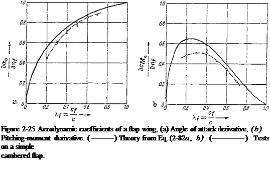
The results of the above formulas are shown in Fig. 2-25. The theoretical relationship between the aerodynamic flap coefficients and the flap chord ratios is well supported by measurements. In Fig. 2-25, the test results of simple cambered flaps by Gothert [21] are added. The deviations are again due to friction effects.

The aerodynamics of flaps and control surfaces will be discussed in more detail in Sec. 8-2-1.

Computation of the velocity distribution on the skeleton line The problem of computing the distribution of circulation and consequently the velocity distribution will now be treated for a given skeleton line shape at a given angle of attack. By introducing Eq. (249) into Eq. (2466), the equation defining the circulation distribution becomes

This is an integral equation for the vortex density к with given values of a — dZ^/dX. It was first solved by Betz [4]. By taking into account the Kutta condition Eq. (2-51) and Eq. (2-50), the velocity distribution about the skeleton profile (see also Fuchs [16]) is given by

For the case of the uncambered profile, = 0, the already known result for the inclined flat plate is valid; see Eq, (2-65). To evaluate the quadrature formula for the velocity distribution, Riegels [49] makes the Fourier substitution

ZW = Zavcosvcp (2-85 a)

V = 1

^ X = |(1 + coscp) (2-856)

Introducing these expressions into Eq. (2-84) makes elementary evaluation of the integrals possible.* The velocity distribution of the skeleton profile is then

where the upper sign is valid for the upper side, the lower sign for the lower side of the skeleton profile. Numerical evaluation of this equation by means of simple quadrature formulas is treated in [49] (see also [28]). The first term of Eq. (2-86) represents the velocity distribution of the inclined flat plate. For the parabolic skeleton

2(5) – — sin2 = t! r — (1 — cos 2ф) c 2 c

[see Eq. (2-68)], = hjc, a% = ~hjc, аъ = a4 = • • ■ = 0. Therefore, Eq. (2-86) yields,

for a = 0,

cos293 — 1 . , . h.

—– – I—— = 1 ^ 4— sing?

smg? c

a result already obtained in Eq. (2-67), taking into account Eq. (2-50).

Velocity and pressure distributions for the skeleton lines of the four – and five-digit NACA profiles, Figs. 2-2a and 2-2b, are given in [1]. In Fig. 2-26 some pressure distributions are presented for the angle of smooth leading-edge flow. For the skeleton lines of the NACA 6-series, pressure distributions have been presented in Fig. 2-23a.

Pressure distribution for given lift coefficient and moment coefficient The problem of approximating a given skeleton line by superposition of an inclined flat plate and a parabolic skeleton in such a way that lift and zero-moment coefficients of approximation and given skeleton are equal can be solved with the help of the above-introduced Fourier series expansion. In this case the Fourier coefficients from Eqs. (2-69) and (2-70) become

12 4

A° = 2wCl + n См° аПС^ =

Figure 2-26 Theoretical pressure distribution of NACA skeleton lines from NACA Rept. 824 at smooth leading-edge flow, (a) Four-digit NACA profile with h/c — 1.0. (b) Five-digit NACA profile with ci$ = 1.0.

These coefficients are introduced into Eq. (2-61), and the resultant distribution, taking into account Eq. (2-53), is obtained as	pressure
	A cp(X) = cLhQ (X) + см о 4h j (X)	(2-87)
with	MX) = !jand MX)=J-(l-4Z)j/!^	(2-88)

The distributions h0(X) and hl(X) are shown in Fig. 2-27.

Bent plate (flap wing) Finally, the pressure distribution of the bent flat plate (flap wing) will be mentioned. For the zero-lift angle of attack, cL = 0, the result is

In Fig. 2-28, the pressure distribution according to this equation is presented for the flap chord ratio Xf = . The cross-hatched area represents the load on the flap, the determination of which as well as that of the flap moment (control-surface moment) will be discussed in Sec. 8-2-1.