Origin of Numerical Dispersion

Let us consider the solution of the simple convective wave equation:

d U d U

+ c = 0 dt dx

and initial condition
t = 0, u(x, 0) = Ф(х).
The Fourier-Laplace transform of (4.11) leads to , 4′ іФ (a) (a 1 (ш — ca) u=——- , (4.12) 2n where U is the Fourier-Laplace transform of u. Ф(a) is the Fourier transform of initial condition u(x, 0). Thus, U is given by
іФ (a) 2п (ш — ca)
(4.13)
The poles of Eq. (4.13) are found by setting the denominator to zero. This yields
ш = ca	(4.14)
which is the dispersion relation. The group velocity or wave speed is given by йш/da. In the case of Eq. (4.11), by using dispersion relation (4.14), the group velocity is
dш da
(4.15)
so that all wave components propagate with the same speed. That is to say, the waves supported by the convective wave equation are nondispersive. Now Eq. (4.11) may be fully discretized by first rewriting it as a system of two equations, each involving only either a temporal or spatial derivative, as follows:
This set of finite difference equations (Eq. 4.16) with discrete variables I and n may be generalized into a set of finite difference equations with continuous variables x

and t. They are as follows:

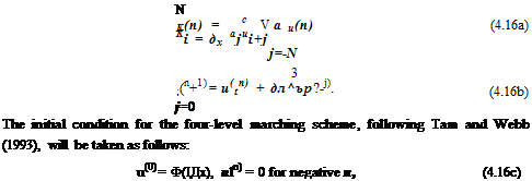
N

K(x, t) =——– ^2 ajU(x + jAx, t) (4.17a)

AX j=-N

3

u(x, t + At) = u(x, t) + At ^2 bjK(x, t — jAt), (4.17b)

j=0

with initial condition

( Ф(x), 0 < t < At

u(x, t) = (4.17c)

I 0, t < 0.

By taking the Fourier-Laplace transform of problem (4.17) and using the Shifting Theorem (see Appendix A), it is straightforward to find, after some algebra, that the solution is

ІФ (a)

2п (ш — ca)

where U is the Fourier-Laplace transform of the solution of the finite difference equation (4.17). Eq. (4.18) is identical to the Fourier-Laplace transform of the solu­tion of the original convective wave equation; i. e., Eq. (4.13), if ш and a in Eq. (4.18) are replaced by ш and a.

The exact solution of the finite difference solution of (4.11) is given by the inverse transform of Eq. (4.18) as follows:

The double integral may be evaluated by first calculating the contributions of the poles in the ш plane. The poles are given by the zeros of the denominator of the integrand, that is, the roots of

ш(ш) = ca(a). (4.20)

Eq. (4.20) is the dispersion relation. This is formally the same as the dispersion relation of the original partial differential equation; i. e., Eq. (4.14), provided ш is replaced by ш and a is replaced by a. For this reason, the finite difference scheme is referred to as dispersion-relation-preserving (DRP).

For a four-level time marching scheme, there would be four poles or Eq. (4.20) has four roots. Let the poles be ш = шj (a), j = 1, 2, 3, 4. One of the poles has Im(«) nearly equal to zero. This is the pole that corresponds to the physical solution. The other poles lead to solutions that are heavily damped.

Numerical dispersion can arise from spatial as well as temporal discretization. Numerical dispersion due to spatial discretization alone will be considered first. For this purpose, the limit At ^ 0 is applied, that is, time is treated exactly. This is

The integrand has a pole at ш = ca(a). On deforming the inverse contour Г to pick up this pole in the ш plane, it is easy to find through the use of the Residue Theorem

TO

u(x, t) = J Ф(a)ei(ax —ш) da. (4.23)

— то ш=са( a)

Now for large t (with x/t fixed), the a-integral of Eq. (4.23) may be evaluated by the method of stationary phase (see Appendix A). The stationary phase point a = as is given by the zero of the derivative of the phase function Ф = (ax/t — ca(a)) with respect to a. This leads to

which yields as as a function of x/t. The asymptotic solution is

where sgn(z) is the sign of z.

Now, ш and a are related by Eq. (4.22). In general, da/da is not a constant equal to 1, so that the group velocity varies with wave number. Different wave numbers of the initial disturbances will propagate with a slightly different speed leading to numerical dispersion.

In the more general case of solution (4.19), when both spatial and temporal dis­cretization are used, the group velocity may be calculated by implicit differentiation of Eq. (4.20). This gives

da

dm = C da da dm

dш

Eq. (4.26) indicates that numerical dispersion can be the result of imperfect spatial discretization, i. e., da/da = 1, or imperfect temporal discretization, i. e., drn/drn = 1. Consideration of imperfect time discretization will be deferred to later because it is quite involved. The effect of dispersion due to spatial discretization will now be illustrated by a numerical example.

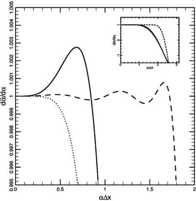
For the convective wave equation (4.11), Eq. (4.24) reveals that the variation in group velocity is caused by the variation of the slope of the a Ax versus a Ax curve. Figure 4.2 shows the da/da versus a Ax curves for the 7-point and 15-point

Figure 4.2. The da/da vs. aAx curves………. , sixth-order central difference scheme; 7-point DRP scheme——– , 15-point DRP scheme.

stencil DRP finite difference schemes. Notice that the da/da curve for the 7-point stencil DRP scheme has a peak at a Ax = 0.67 at which da/da = 1.00276. That is, the wave component with a Ax = 0.67 (wave with 9.38 mesh points per wavelength) will propagate faster than the exact wave speed da/da = 1.0 by about 0.3 percent. Suppose, in a computation, the waves propagate over a distance of 400 mesh points. In this case, when the main part of the wave packet reaches x = 400, the wave com­ponent with a Ax = 0.67 will reach x = 401.1. Under these circumstances, numerical dispersion would just be noticeable as wave dispersion exceeds one mesh point. On the other hand, if the standard sixth-order scheme is used instead, severe numerical dispersion will result when the main wave reaches x = 400. Waves in the wave num­ber range of a Ax > 0.6, having a group velocity less than 1.0, would form trailing waves.

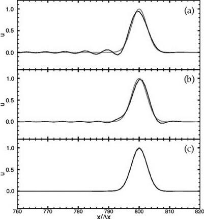
A relevant question to ask is how to reduce numerical dispersion due to spatial discretization. This can be done by using a scheme with a larger stencil. Figure 4.2 shows the da/da curve for the 15-point stencil DRP scheme. For aAx < 1.73, the group velocity differs from 1.0 by no more than 0.1 percent. Thus, if the wave packet of the solution contains only waves with wave number aAx < 1.73, then there will be no observable numerical dispersion even after the wave packet propagates over a distance of up to 1000 mesh points. As a concrete example, Figure 4.3 shows the

Figure 4.3. Comparisons between computed solutions and exact solution for the one­dimensional convective wave equation. (a) sixth-order central difference scheme; (b) 7-point DRP scheme; (c) 15-point DRP scheme.

computed solution of the convective wave equation (4.11) with initial condition in the form of a Gaussian with a half-width of 3 mesh spacings,

u(x, 0) = e-(ln2)()2,

using the standard sixth-order scheme, the 7-point stencil, and the 15-point stencil DRP scheme. It is easy to see that there is significant numerical dispersion (with extensive trailing waves) when computed by the standard sixth-order scheme. The 7-point stencil DRP scheme is better. Both schemes, having the same stencil size, require the same amount of computation. The solution by the 15-point stencil is even better. For all intents and purposes, the solution is identical numerically to the exact solution.