Rotor thrust, inflow, Zw and vertical gust response in hover

The rotor thrust T in hover can be determined from the integration of the lift forces on the blades

(2.53)

Using eqns 2.17-2.21, the thrust coefficient in hover and vertical flight can be written

as

(2.54)

Again, we have assumed that the induced downwash ki is constant over the rotor disc; Hz is the normal velocity of the rotor, positive down and approximates to the aircraft velocity component w. Before we can calculate the vertical damping derivative Zw, we need an expression for the uniform downwash. The induced rotor downwash is one of the most important individual components of helicopter flight dynamics; it can also be the most complex. The downwash, representing the discharged energy from the lifting rotor, actually takes the form of a spiralling vortex wake with velocities that vary in space and time. We shall give a more comprehensive treatment in Chapter 3, but in this introduction to the topic we make some major simplifications. Assuming that the rotor takes the form of an actuator disc (Ref. 2.17) supporting a pressure change and accelerating the air mass, the induced velocity can be derived by equating the work done by the integrated pressures with the change in air-mass momentum. The hover downwash over the rotor disc can then be written as

(2.55)

where Ad is the rotor disc area and p is the air density. Or, in normalized form

(2.56)

The rotor thrust coefficient Ct will typically vary between 0.005 and 0.01 for heli­copters in 1 g flight, depending on the tip speed, density altitude and aircraft weight. Hover downwash ki then varies between 0.05 and 0.07. The physical downwash is
proportional to the square root of the rotor disc loading, Ld, and at sea level is given

by

Vihover = 14-VLd (2.57)

For low disc loading rotors (Ld = 6 lb/ft2, 280N/m2), the downwash is about 35 ft/s (10 m/s); for high disc loading rotors (Ld = 12 lb/ft2, 560 N/m2), the downwash rises to over 50 ft/s (l5 m/s).

The simple momentum considerations that led to eqn 2.55 can be extended to the energy and hence power required in the hover

T3/2

Pi = T Vi = ——————-

i i V(2Md)

The subscript i refers to the induced power which accounts for about 70% of the power required in hover; for a 10000-lb (4540 kg) helicopter developing a downwash of 40 ft/s (typical of a Lynx), the induced power comes to nearly 730 HP (545 kW). Equations 2.54 and 2.56 can be used to derive the heave damping derivative

where

d Ct 2a0s ki

d^z 16ki + a^s

and hence

where Ab is the blade area and s the solidity, or ratio of blade area to disc area. For our reference Helisim Lynx configuration, the value of Zw is about —0.33/s in hover, giving a heave motion time constant of about 3 s (rise time to 63% of steady state). This is typical of heave time constants for most helicopters in hover. With such a long time constant, the vertical response would seem more like an acceleration than a velocity type to the pilot. The response to vertical gusts, wg, can be derived from the first-order approximation to the heave dynamics

dw

——— Zww = Zww

dt

The initial acceleration response to a sharp-edge vertical gust provides a useful measure of the ride qualities of the helicopter, in terms of vertical bumpiness

A gust of magnitude 30 ft/s (10 m/s) would therefore produce an acceleration bump in Helisim Lynx of about 0.3 g. Additional effects such as the blade flapping, downwash lag and rotor penetration will modify the response. Vertical gusts of this magnitude

are rare in the hovering regime close to the ground, and, generally speaking, the low values of Zw and the typical gust strengths make the vertical gust response in hovering flight fairly insignificant. There are some important exceptions to this general result, e. g., helicopters operating close to structures or obstacles with large downdrafts (e. g., approaching oil rigs), that make the vertical performance and handling qualities, such as power margin and heave sensitivity, particularly critical. We shall return to gust response as a special topic in Chapter 5.

The coefficient outside the parenthesis in eqn 2.67 is the expression for the correspond­ing value of heave damping for a fixed-wing aircraft with wing area Aw.

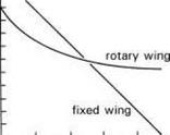
The key parameter is again blade/wing loading. The factor in parenthesis in eqn 2.67 indicates that the helicopter heave damping or gust response parameter flattens off at high-speed while the fixed-wing gust sensitivity continues to increase linearly. At lower speeds, the rotary-wing factor in eqn 2.67 increases to greater than one. Typical values of lift curve slope for a helicopter blade can be as much as 50% higher than a moderate aspect-ratio aeroplane wing. It would seem therefore that all else being equal, the helicopter will be more sensitive to gusts at low-speed. In reality, typical blade loadings are considerably higher than wing loadings for the same aircraft weight; values of 100 lb/ft2 (4800 N/m2) are typical for helicopters, while fixed-wing executive transports have wing loadings around 40 lb/ft2 (1900 N/m2). Military jets have higher wing loadings, up to 70 lb/ft2 (3350 N/m2) for an aircraft like the Harrier, but this is still quite a bit lower than typical blade loadings. Figure 2.28 shows a comparison of heave damping for our Helisim Puma helicopter (a0 = 6, blade area = 144 ft2 (13.4 m2)) with a similar class of fixed-wing transport (a0 = 4, wing area = 350 ft2 (32.6 m2)), both weighing in at 13 500 lb (6130 kg). Only the curve for the rotary-wing aircraft has been extended to zero speed, the Puma point corresponding to the value

0.2 г

0.0 –

0.5

-0.4

-0.&

-0.8 -1.0

40 60 80 100 airspeed Im/s)

Fig. 2.28 Variation of heave damping, Zw, with airspeed for rotary – and fixed-wing aircraft

of Zw given by eqn 2.61. The helicopter is seen to be more sensitive to gusts below about 50 m/s (150 ft/s); above this speed, the helicopter value remains constant, while the aeroplane response continues to increase. Three points are worth developing about this result for the helicopter:

(1) The alleviation due to blade flapping is often cited as a major cause of the lower gust sensitivity of helicopters. In fact, this effect is fairly insignificant as far as the vertical gust response is concerned. The rotor coning response, which determines the way that the vertical load is transmitted to the fuselage, reaches its steady state very quickly, typically in about 100 ms. While this delay will take the edge off a truly sharp gust, in reality, the gust front is usually of ramp form, extending over several of the blade response time constants.

(2) The Zw derivative reflects the initial response only; a full assessment of ride qualities will need to take into account the short-term transient response of the helicopter and, of course, the shape of the gust. We shall see later in Chapter 5 that there is a key relationship between gust shape and aircraft short-term response that leads to the concept of the worst case gust, when there is ‘tuning’ or ‘resonance’ between the aircraft response and the gust scale/amplitude.

(3)

The third point concerns the insensitivity of the response with speed for the helicopter at higher speeds. It is not obvious why this should be the case, but the result is clearly connected with the rotation of the rotor. To explore this point further, it will help to revisit the thrust equation, thus exploiting the modelling approach to the full:

where

Ut ~ r + д sin ф, Up = ptz — k; — дв cos ф — rв (2.70)

The vertical gust response stems from the product of velocities Up Ut in eqn 2.69. It can be seen from eqn 2.70 that the forward velocity term in Ut varies one-per-rev, therefore contributing nothing to the quasi-steady hub loading. The most significant contribution to the gust response in the fuselage comes through as an N – per-rev vibration superimposed on the steady component represented by the derivative Zw. The ride bumpiness of a helicopter therefore has quite a different character from that of a fixed-wing aircraft where the lift component proportional to velocity dominates the response.