THE REYNOLDS NUMBER

Experimental work published by Osborne Reynolds in 1883 showed that there are two distinct types of flow, laminar and turbulent. These may change from one to the other according to particular conditions. Which type of flow prevails in the boundary layer at any point depends on the form, waviness and roughness of the surface, the speed of the mainstream measured at a distance from the surface itself, the distance over which the flow has passed on the surface, and the ratio of density to viscosity of the fluid. A variation in any Of these factors can bring about a change in the boundary layer. Reynolds combined them all except surface condition, into one figure, the Reynolds number. The formula for Reynolds number is:

Reynolds Number, Re = Viscosity x Velocity x Length

, , . . , , „ « „ , pVL V x L

In the standard symbols: Re = x V x L or—————— or———-

Ц ft v

(The Greek letter v ‘nu’ stands here for the kinematic viscosity of the fluid)

Viscosity is measured in kilogrammes per metre per second, the standard value for air is 17.894 x 10-6 or.0000179 kg/m/sec (.373 X 10-6 slugs/fl/sec). As the equation shows, as viscosity increases, Reynolds number decreases. The average Re of a model wing or tail surface may be found using the normal flying speed as the velocity and the average chord as the length, so, for example, a wing of chord 0.1 metres flying at 10 metres per second with standard density and viscosity has Re (1.225/.000017894) x 0.1 x 10 = (68459) x 1 — 68459. A useful abbreviation for most modelling needs is thus provided by the simplified equation:

Re = 68459 x VL

where V and L are in m/sec and metres. If V and L are in ft/sec and feet, Re = 6363 x VL. As density, velocity and length increase, Reynolds number increases. It is often suggested that since density and viscosity are not under control, for modelling purposes the VL figure alone is important and in most ways this is true providing it is remembered that the VL is expressed in units (metres x metres/sec., or ft x ft/sec.) whereas the Re is non – dimensional. For a fuller understanding of Re effects, however, the ratio of inertia forces to viscosity forces in the boundary layer is what counts, relative to the speed of flow at each point This ratio (toes vary appreciably according to seasonal conditions and altitude. Reynolds numbers rise in winter. (See Appendix 1).

3.2 TYPICAL AVERAGE REYNOLDS NUMBERS

Aircraft type

Commercial aircraft Light aeroplane

Sailplane at max. speed, wing root Sailplane at min. speed, wing tip

Pylon racing model aeroplane at max. speed

Hang gliders, man-powered aircraft, ultra light aeroplanes

Multi-task R. C. sailplanes in speed task: when soaring:

Large model sailplanes Thermal soaring: penetrating:

A-l, A-2 sailplanes, Wakefields, Coupe d’Hiver etc. max.

min.

Indoor models, ‘peanut’ scale etc.

Large soaring bird, (e. g. albatross or eagle) Seagull

Butterfly (gliding) 7,000

(The above figures are all approximate and depend on the actual speeds of flight, wing chords, etc.)

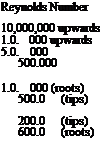
Typical values of Re for various types of model are shown in the table. It is important to remember that the chord of a wing tip is usually smaller than the root, so the Re is less. For the example model with Re average about 68000, the tip chord might be 0.08 metres and the root 0.12, so the Re at each would be about 48000 and 81000. This is of special importance for the phenomenon of wing tip stalling in models.

No model flies at constant speed for long. Each change of speed alters the Re, in simple proportion. The faster the flight, the higher the Reynolds number. If the tailplane has smaller chord than the wing, the operating Re will be less for the tail.