Numerical Dispersion Arising from Temporal Discretization

As pointed out in Section 4.3, computation schemes that have a DRP property will exhibit numerical dispersion due to temporal discretization if dm/dm of the angular frequency relationship m(m) is not equal to 1.0 (see Tam, 2004). Most single time step
schemes, such as the Runge-Kutta method, do not have a DRP property. However, they do lead to numerical dispersion. For schemes of this type, there is no general way to derive the dispersion relation. To illustrate this point, consider again the numerical solution of the convective wave equation (4.11) by finite difference. Suppose the 15-point stencil DRP scheme is used to approximate the spatial derivative. This spatial scheme can accurately resolve waves with as few as 3.6 mesh points per wavelength so that, unless an acoustic pulse has extremely narrow half-width, there is negligible dispersion due to spatial discretization. This leaves any observed numerical dispersion to come primarily from temporal discretization. The Fourier transform of the discretized form of Eq. (4.11) is

f = f(u >. (4-27a)

where f (й) = – ica(a)U. (4.27b)

Now suppose the time derivative of Eq. (4.27a) is discretized by the fourth-order Runge-Kutta scheme with time step At (see Eq. (3.2)). It is straightforward to find that the time marching finite difference equation for й(п) is

4

1 + ^2 cj (-icaAt)) j=1

Eq. (4.28) is a first-order finite difference equation in n. It can be readily generalized into a finite difference equation with a continuous variable. By applying the Laplace transform to the difference equation, it is easy to determine that the dispersion relation of the finite difference algorithm of the convective wave equation discretized temporally by a fourth-order Runge-Kutta scheme is

4

1 + ^2 Cj (-icaAt))

j=1

By differentiating Eq. (4.29) with respect to a, the following formula for the group velocity is derived:

(4.30)

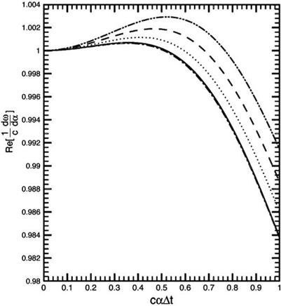
Since dm/da is not a constant equal to c even if da/da = 1.0, numerical dispersion is introduced by the use of the Runge-Kutta scheme. A plot of Re(dm/da) as a function of caAt (a = a assumed) for the low-dissipation low-dispersion Runge – Kutta (LDDRK) scheme is given as one of the curves in Figure 4.5. Notice that the group velocity drops below c for caAt > 0.5. The group velocity is less than the exact wave speed by at least 0.2 percent for caAt > 0.65. Waves in this range will form trailing waves.

To illustrate numerical dispersion due to temporal discretization, consider com­puting the solution of Eq. (4.11) with initial condition,

using the 15-point stencil DRP scheme for spatial discretization and the standard fourth-order Runge-Kutta scheme for temporal discretization. For convenience, the wave speed c is set equal to unity. The computed results are shown in Figure 4.4. Figure 4.4a shows the computed waveform after the pulse has propagated a distance of 608 mesh spacings using a very small time step At = 0.25Ax. The computed result is indistinguishable from the exact solution. Figure 4.4b shows the computed result when a larger At, At = 0.76Ax, is used. There is no question that the pulse is slightly dispersed. The cause is temporal discretization. For comparison purposes, Figure 4.4c shows the computed waveform using the LDDRK scheme of Hu et al. (1996) with At = 0.76Ax. There is definitely an improvement with the use of this scheme. However, there are still some trailing waves, a manifestation of numerical dispersion. For the initial condition (4.31), a small fraction of the initial pulse has

Figure 4.5. Optimized group velocity of the convective wave equation.———— , n = 0.6; …… , n = 0.7;—————— , n = 0.8; …………… , n = 0.9;———- , Hu et al. (1996) LDDRK scheme.

a wave number larger than a Ax = 0.855 corresponding to a At = 0.65. This part of the initial spectrum will propagate slower according to the group velocity curve of Figure 4.5. They show up as trailing waves. Finally, Figure 4.4d shows the computed result of the four-level time marching DRP scheme. The four-level scheme computes the derivative function once per step. The single step Runge-Kutta scheme computes the derivative function four times per step. Thus, to compare the results based on nearly the same workload, the time step of the DRP scheme is taken to be a quarter of that of the Runge-Kutta scheme, i. e., At = 0.19Ax. As can be seen, the results of Figures 4.4b, 4.4c, and 4.4d seem to indicate that the DRP scheme has less dispersion due to temporal discretization.

For certain wave propagation problems, minimizing dispersion error could be an important consideration. To do so, one might choose the free parameters or constants of the Runge-Kutta scheme to minimize the difference between the group velocity and the exact velocity of propagation of the governing wave equation. For the simple convective wave equation, the group velocity is given by Eq. (4.30). Suppose in (4.28) c1 and c2 are given the values of 1.0 and 0.5, but allow c3 and c4 to be free parameters. These parameters are then chosen to minimize the square of

n	c3	c4
0.6	0.163168	4.07351 E-02
0.7	0.161940	4.04090 E-02
0.8	0.160545	4.00390 E-02
0.9	0.158992	3.96280 E-02
Hu et al. (1996)	0.162997	4.07574 E-02
Standard fourth-order RK	0.166667	4.16667 E-02

Table 4.1. Values of parameter c3 and c4

the difference between the group velocity and the exact wave speed c = 1 over a band of wave number. It will be assumed that the spatial discretization is exact; i. e., a = a. Thus, c3 and c4 are chosen to minimize the integral,

Table 4.1 gives the values of c3 and c4 for different choices of n. The group velocity Re (dm/da) as a function of caAt corresponding to these choices of c3 and c4 is plotted in Figure 4.5. It is clear from this figure that by using a large n the minimization procedure forces a large band of wave number to have a group velocity closer to c. However, it is a feature of mean squared minimization that this also leads to a larger overshoot. So one might select a compromise between a larger bandwidth with a normalized group velocity closer to 1.0 and a smaller overshoot. Plotted also in Figure 4.5 is the group velocity curve of the LDDRK scheme. It turns out that it is almost identical to that of the choice n = 0.6. This is strictly a coincidence! But this appears to offer an explanation of why the LDDRK scheme does not incur excessive numerical dispersion error arising from temporal discretization.