Vector-differential form of equations of motion

Returning now to the general linear problem, we shall find it convenient to use the vector-matrix shorthand form of the equations of motion, written in the form

dx

—— Ax = Bu + f(t) (2.71)

dt

where

x = {u, w, q, 9, v, p, ф, r, ф}

A and B are the matrices of stability and control derivatives, and we have included a forcing function f(t) to represent external disturbances, e. g., gusts. Equation 2.71 is a linear differential equation with constant coefficients that has an exact solution with analytic form

t

x(t) = Y(t) x(0) + у Y(t — t ) (Bu + f(T)) dr 0

Y(t) = 0, t < 0

Y(t) = U diag[exp(kft)]U—1, t > 0 (2.72)

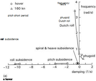
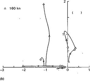
The response behaviour is uniquely determined by the principal matrix solution Y(t) (Ref. 2.18), which is itself derived from the eigenvalues kf and eigenvectors u; (ar­ranged as columns in the matrix U) of the matrix A. The stability of small motions about the trim condition is determined by the real parts of the eigenvalues and the complete response to controls u or disturbances f is a linear combination of the eigenvectors. Figures 2.29(a) and (b) show how the eigenvalues for the Helisim Lynx and Helisim Puma configurations vary with speed from hover to 160 knots; at the higher speeds, the conventional fixed-wing parlance for naming the modes associated with the eigenval­ues is appropriate. The pitch instability at high speed for the hingeless rotor Helisim Lynx has already been discussed in terms of the loss of manoeuvre stability. At lower speeds the modes change character, until at the hover they take on shapes peculiar to the helicopter, e. g., heave/yaw oscillation, pitch/roll pendulum mode. The heave/yaw mode tends to be coupled, due to the fuselage yaw reaction to changes in rotor torque, induced by perturbations in the rotor heave/inflow velocity. The eigenvectors represent the mode shapes, or the ratio of the response contributions in the various DoFs. The

damping (1 Is)

Fig. 2.29 (a) Variation of Lynx eigenvalues with forward speed; (b) variation of Puma
eigenvalues with forward speed

modes are linearly independent, meaning that no one can be made up as a collection of the others. If the initial conditions, control inputs or gust disturbance have their energy distributed throughout the DoFs with the same ratio as a particular eigenvector, then the response will be restricted to that mode only. More discussion on the physics of the modes can be found in Chapter 4.

The key value of the linearized equations of motion is in the analysis of stability; they also form the basic model for control system design. Both uses draw on the considerable range of mathematical techniques developed for linear systems analysis. We shall return to these later in Chapters 4 and 5, but we need to say a little more about the two inherently nonlinear problems of flight mechanics – trim and response.

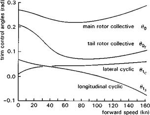
Fig. 2.30 Variation of trim control angles with forward speed for Puma

The former is obtained as the solution to the algebraic eqn 2.2 and generally takes the form of the controls required to hold a steady flight condition. The general form of control variations with forward speed is illustrated in Fig. 2.30. The longitudinal cyclic moves forward as speed increases to counteract the flapback caused by forward speed effects (Mu effect). The lateral cyclic has to compensate for the rolling moment due to the tail rotor thrust and also the lateral flapping induced in response to coning and longitudinal variations in rotor inflow. The collective follows the shape of the power required, decreasing to the minimum power speed at around 70 knots then increasing again sharply at higher speeds. The tail rotor collective follows the general shape of the main rotor collective; at high-speed the pedal required decreases as some of the anti-torque yawing moment is typically produced by the vertical stabilizer.

While it is true that the response problem is inherently nonlinear, it is also true that for small perturbations, the linearized equations developed for stability analysis can be used to predict the dynamic behaviour. Figure 2.31 illustrates and compares the pitch response of the Helisim Lynx fitted with a standard and soft rotor as a function of control input size; the response is normalized by the input size to indicate the degree of nonlinearity present. Also shown in the figure is the normal acceleration response; clearly, for the larger inputs the assumptions of constant speed implicit in any linearization would break down for the standard stiffer rotor. Also the rotor thrust would have changed significantly in the manoeuvre and, together with the larger speed excursions for the stiffer rotor, produce the nonlinear response shown.