Finite Difference Solution of the Linearized Euler Equations

5.1 Dispersion Relations and Asymptotic Solutions of the Linearized Euler Equations

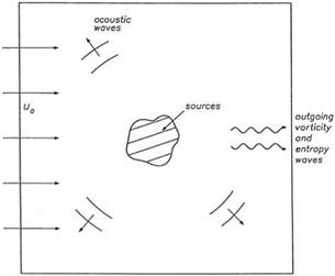
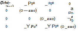
Consider small-amplitude disturbances superimposed on a uniform mean flow of density p0, pressure p0, and velocity u0 in the x direction (see Figure 5.1). The linearized Euler equations for two-dimensional disturbances are as follows:

d U 9 E 9 F

dt dx dy

where

	p		P0U + p U0		p0v
	u		U0U + p		0
U=		, E =	0 p0	, F =	p P0
	v		u0v
	p		U0 P + Y P0U_		Y p0v

The nonhomogeneous term H on the right side of Eq. (5.1) represents distributed time-dependent sources.

The Fourier-Laplace transform f (а, в, *) of a function f(x, y, t) is related to the function by

to to

f(a, e,v) = II I f (x, y, t)e-i(ax+ey-*)dxdydt

0 —to

TO

f (xy-‘) = f(a-f>-^e’-"da de d*

Г —to

In these equations, the contour Г is a line parallel to the real axis in the complex * plane above all poles and singularities of the integrand (see Appendix A).

Now, consider the general initial value problem governed by the linearized Euler equation (5.1). The initial condition at t = 0 is

u = “initial (x, y)- (5.2)

Figure 5.1. Sources of acoustic, vortic – ity, and entropy waves in a uniform flow.

The general initial value problem for arbitrary nonhomogeneous source term H can be solved formally by Fourier-Laplace transforms. As shown in Appendix A, the Laplace transform of a time derivative is

The Fourier-Laplace transform of Eq. (5.1) is a system of linear algebraic equations that may be written in the following form:

AU — G,

where

and i[H )] represents the sum of the transforms of the source term

and the initial condition.

It is easy to show that the eigenvalues X and eigenvectors Xj (j — 1, 2, 3, 4) of matrix A are

X1 — X2 — (o au0)

X3 — (o — aU0) + $0 (a + в ) X4 — (o — au0) — a0 (a2 + в2)

where a0 = (yp0/p0)1/2 is the speed of sound. The solution of Eq. (5.4) may be expressed as a linear combination of the eigenvectors as follows:

The coefficient vector C, having elements Cj (j = 1 to 4), is given by

C = X-1G. (5.10)

X 1 is the inverse of the fundamental matrix:

Eq. (5.9) represents the decomposition of the solution into the entropy wave, X1, the vorticity wave, X2, and the two modes of acoustic waves, X3 and X4. Now, each wave solution will be considered individually.

5.1.1 The Entropy Wave

The entropy wave consists of density fluctuations alone; i. e., u = v = p = 0. By inverting the Fourier-Laplace transform, it is straightforward to find that p is given by

TO

p(x, y, t) = [ [ [ ———– C—— e'(ax+ey—ot’ida de dox (5.12)

J J J (o – au0)

Г —то

The zero of the denominator gives rise to a pole of the integrand. The relationship between o, a, and в arising from this zero is the dispersion relation. In this case, it is

X1 = (o — au0) = 0. (5.13)

C1 may have poles in the o plane. This is due to periodic forcing. If the wave is excited by initial condition alone, then C1 is independent of o.

In the a plane, the zero of the integrand of Eq. (5.13) is given by

a = — (Im (o) > 0 when o is on Г).

u0

The a-integral of Eq. (5.12) may now be evaluated by means of the Residue Theorem. For x > 0, Jordan’s Lemma requires the completion of the contour on the top half

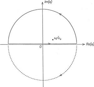Figure 5.2. Inversion contours and pole in the complex a plane.

a plane as shown in Figure 5.2. For x < 0, the contour is completed in the lower half-plane. Thus,

5.1.2 The Vorticity Wave

The vorticity wave consists of velocity fluctuations alone. That is, there are no

The integral in Eq. (5.16) may be evaluated in the same way as that in Eq. (5.12). This leads to

x(x – u0t, y) x ^ TO 0, x ^ —to

Just as for entropy waves, the vorticity wave is convected downstream as a frozen pattern at the speed of the mean flow.