Modelling of Uncertainties in Parameters

We assume that the free-stream turbulence in the atmosphere randomly and simul­taneously changes the velocity vector or, what is equivalent the Mach number Eq. 4 and the angle of attack Eq. 3. One should not mix this kind of turbulence with the turbulence in the boundary layer reasoned by friction. It is assumed that turbulence vortices in the atmosphere are comparable with the size of the airplane. The free – stream turbulence in the atmosphere is modelled by two additionally axes-parallel velocity vectors v1 := v1(91) and v2 := v2(Q2) (Fig. 1), which have Gaussian distri­bution [13]. We model the free-stream turbulence via two random vectors (in 3D it will be three vectors) vi and v2 which change a and Ma (see Fig. i):

o9i ов2

Vl = ~/2 an^ V2 = ~/2′

where 91 and 92 are two Gaussian random variables with zero mean and unit vari­ance, a := Iu„, I the mean turbulence intensity and u«, the undisturbed free stream velocity beyond the boundary layer. This mean turbulence intensity is often used for characterising turbulence in a wind tunnel. For instance, I = 0.001 means low turbulence, I = 0.002 middle and I = 0.005 high turbulence.

Denoting

9 := J9f + 9}, v := sj\ + /3 := arctg^ and г := ^L, (2)

and performing easy geometrical computations, obtain the new angle of attack and the new Mach number:

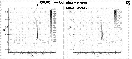
Fig. 2 (left) The difference Ap := |p — p| between the deterministic density p := p(ot, Ma) and the mean density p. (right) The same is for the pressure Ap := p — p. Here p Є (0.5,1.2) and p є (0.7,1.3).

/ J_^ і—

Ma (0i,02) = May 1 H—————- v2l0cos(/3 + a). (4)

Further we study how uncertainties in a and Ma spread into the solution. We note that uncertainties in a and in Ma can be modelled in a different way (see e. g. [23], [27]). >From the construction one can see that Ma := E(Ma (01,02)) and a := E(af (01,02)) are equal to the deterministic values Ma and a, here E(-) is the mathematical expectation. In Fig. 2 (left) we compare the deterministic dens­ity p(a, Ma) with the p := E(p(a (0i, 02),Ma (0i, 02))) for the Case 9 (a = 2.79, Ma := 0.734). In Fig. 2 (right) we do the same comparison for the deterministic pressure. One can see a large difference in the shock position. This large difference motivates us to model uncertainty in a and in Ma.