The Acoustic Wave

The acoustic waves involve fluctuations in all the physical variables. The dispersion relation is given by

Л3Л4 = (ш – au0)2 – «0(a2 + в2) = 0. (5.17)

The formal solution may be found by inverting the Fourier-Laplace transforms. After some algebra, the formal solution may be written as

еі(ах+ву—ш)da dp dm.

(5.18)

(5.19)

Now, the integrals of Eq. (5.18) will be evaluated in the limit (x2 + y2) ^ to. The в – integral will be evaluated first. The poles in the в plane are at p± which are given by

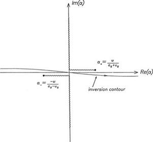
The branch cuts of this square root function in the a plane are taken to be

where the left (right) equality sign is to be used when ш is real and positive (negative). The branch cut configuration and the position of the inverse a-contour are shown in Figure 5.3. This configuration is valid regardless whether ш is real and positive or negative. In the в plane the integrand of Eq. (5.18) has a simple pole at в± in the upper half-plane and a simple pole at в_ in the lower half-plane (see Figure 5.4). For y > 0 (y < 0), the inversion contour may be closed in the upper (lower) half­plane by adding a large semicircle as shown (by Jordan’s lemma). By invoking the

Figure 5.3. The branch cut configuration and inversion contour in the complex a plane.

Residue Theorem, the expressions for p and p simplify to

(5.22)

In Eq. (5.22), r and в are the polar coordinates and Ф = a cose + i[a2 – (m – aw0)2/a2 ]1/2 sine.

In the far field, where r ^ to, the а-integral of Eq. (5.22) can be evaluated by the method of stationary phase (see Appendix B). A straightforward application of this method gives

2n

r |Ф"|

Figure 5.4. The poles and inversion con­tour in the complex в plane.

where as is the stationary phase point, вs = в+(as), Ф" (as) = й2Ф/йа2а=а, and V^) = nocos0 + a0(1 – u0 sin20/fl2)i/2. Eq. (5.23) may be rewritten in the more convenient form:

Similarly, the integrals for u and v can be evaluated. The complete asymptotic solution has the following form:

where

V(в) = u0cosв + a0(1 – M2sin2 в)2; M = u0/a0

„ cos в – M(1 – M2sin2 в)1/2 u^’) (1 – M2sin2 в)1/2 – M cos в

v(0) = sin в[(1 – M2sin2 в)2 + Mcos в].

V(0) is the effective velocity of propagation in the в – direction. This asymptotic solution and that of the entropy and vorticity waves will become useful later.