Trailing-Edge Noise Model

The corresponding PSD of the far-field sound reads

„ , . (кхз Lc 2 ш

Spp(x, w) = (iTSir) c J_По(U, k* (17)

It is written here in non-dimensional variables, introducing the wavenumber spectrum of the wall-pressure fluctuations

По(Ш, к*) = – Фрр(ш) £y(к*,ш),

U c п

where Фрр(ш) is the wall-pressure PSD induced closely upstream of the trailing edge by the incident turbulence only (ignoring contamination by the Kutta condition) and £y(k*,u>) is the correlation length defined from the coherence function between two span-wise locations щ apart from each other as

£y (k*,ш)= у/72(П2,ш) cos(k2 П2) d^2 .

о

The associated long-span approximation reads

The key practical issue is to get a relevant information on Фрр(^) and £y(Щ, ш). Very different flow conditions are encountered in engineering applications, corresponding to different wall-pressure statistics: attached turbulent boundary layers with more or less pronounced adverse pressure gradients, intermittently separated flows, re-attached flows after leading – edge separation and so on (in principle separated flows are out of the scope of usual trailing-edge noise modeling, except if the trace of the turbulence in terms of wall pressure still exhibits a phase convection speed in the stream- wise direction). The source information is reconstructed in experimental studies by interpolation from measurements on a cluster of wall-pressure sensors. Span-wise distributed sensors are needed to give partial access to the correlation length, and chord-wise sensors are needed to evaluate the convection speed Uc involved in the transfer function I. When small-scale mock-ups are tested in wind tunnels, the size of the sensors causes resolution issues that limit the relevance of the measurements; furthermore very thin areas such as the vicinity of the trailing edge are difficult to implement. This makes eq. (17) and eq. (18) more difficult to feed with reliable input data when compared to the equivalent expressions for turbulence-impingement noise.

Caution is required if Computational Fluid Dynamics is used to simulate the flow. At moderate Mach numbers, incompressible LES is the minimum required computational effort, but it may be not affordable. A possible alternative is resorting to RANS (Reynolds-Averaged Navier-Stokes) com­putations to infer the inner and/or outer scales of the boundary layers, and reconstructing the quantities Фрр and £y via empirical laws previously tuned on experimental data bases. This approach still needs being com­forted, facing the wide variety of possible flows encountered in rotating blade technology. Furthermore wall-pressure fluctuations are caused by turbulent patterns developing at different heights in the boundary layer and traveling at different convection speeds. Larger and faster eddies are farther away from the wall whereas smaller and slower ones are convected at shortest distance. In the same time larger or smaller eddies define lower or higher frequencies at same convection speed. This intricate mechanisms make the wall-pressure statistics difficult to analyze. Schematically arbitrary low fre­quencies can be produced by small-scale turbulence convected at very low speed. But eddy size is limited by boundary layer thickness, so that the correlation length is expected to drop at vanishing frequencies.

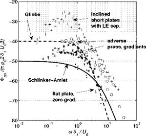
Wall pressure statistics is addressed more specifically in chapter 6. Com­plementary considerations are presented in the present section for trailing – edge noise applications. Wall-pressure spectra Фрр measured beneath bound­ary layers over flat plates and/or curved airfoil surfaces with more or less pronounced stream-wise pressure gradients are first reported in Fig. 13 in dimensionless variables taking the displacement thickness as parameter. For finite-chord airfoils the measurement has been performed close to the trail­ing edge. Developed turbulence over a flat plate with zero pressure gra­dient (small dots) often taken as reference is found to produce the lowest fluctuations. In contrast an adverse pressure gradient causes a significant increase, more especially at lower frequencies, up to 10 or 20 dB. This has been observed by many investigators, on both large plates and airfoils, and certainly depends on many parameters, such as curvature and gradient strength. More especially leading-edge separation followed by reattachment is found to produce the highest levels, with a wide low-frequency bump. This flow regime is typical of thin or roughly designed leading-edges in fan – noise technology, for which off-design conditions can be encountered.

Figure 13. Wall-pressure spectra measured beneath tur­bulent boundary layers, with or without pressure gradient, made dimensionless by outer variables, from Keith et al (1992) and ECL flat-plate data. External-variable models plotted for comparison.

Model wall-pressure spectra can be built up based on boundary-layer parameters. A review dedicated to aeronautical fan-noise applications has

been proposed for instance by Gliebe et al (2000). Substantial differences might be expected for low-speed cooling fans. First reported attempts for the definition of universal statistical models are based on the use of outer boundary-layer variables to scale the wall-pressure spectrum, as

where the second form is directly expressed in terms of frequency. Schlinker – Amiet’s model reads

Фрр(ш) = 10-5 (1+ ш +0.217Ш2 +0.00562а4)-1, ш = ш51/и0

and Gliebe’s et al model

Фрр(ш) = 10-4 (1 + аш2) 5/2 ,

where а is 0.5 in the reference, and is better replaced by a smaller value, here 0.3 to fit with the low-Mach number results of Fig. 13. Both provide constant values at vanishing frequencies, abusive in view of some measure­ments, and asymptotic high-frequency trends like ш-4 and ш-5. The former and the latter hold for zero and adverse pressure gradients, respectively. The alternative Chase-Howe model based on inner variables (not plotted here) is expressed as

where тр is the wall-shear stress. It is known to yield better high-frequency collapse and reproduces some low-frequency decrease. In counterpart the wall-shear stress is of more difficult access for practical applications. The large scatter of data in Fig. 13 suggests that model predictions could be very sensitive to the pressure gradient associated with aerodynamic loading. Yet this gradient does not enter explicitly the definition of aforementioned models. An improved model including the pressure gradient and based on mixed variables has been proposed very recently by Rozenberg et al (2012). The assessment on extended sets of experimental data still requires further investigation.

The correlation length is another matter of concern for sound predictions. For developed turbulence in boundary layers with zero pressure gradient,

Corcos’ model is often used. The corresponding expression reads

u/(bcUc)

Щ + u2/(bcUc)2 ’

where bc is a constant, and essentially states that the correlation is inversely proportional to frequency (at least for parallel gusts k2 =0). This property is not physically consistent at very low frequencies. Indeed low frequencies naturally correspond to large scales and scales larger than the boundary layer thickness cannot be found.

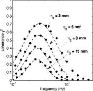
Figure 14. Evidence of a log-normal distribution of the span-wise coherence as a function of frequency. Left: measured data on a thin, moderately cambered rotating blade, from Rozenberg et al (2008). Right: reference data of Brooks & Hodgson (1981).

Evidence of a relevant Gaussian distribution of the coherence as a func­tion of frequency on a logarithmic scale is reported in Fig. 14. The left-hand side plot refers to wall-pressure measurements directly made on the blades of a low-speed axial fan, from Rozenberg et al (2008). They are compared to a theoretical fit that obeys the log-normal law

in which the parameters A, f0, a appear as functions of the span-wise sep­aration. Only retaining the variations of A as dominant makes the same
qualitative variations expected for the correlation length. A similar be­havior is reported by Roger & Moreau (2004) about the development of a rapidly growing boundary layer close to the trailing edge of a Controlled – Diffusion airfoil, in a flow regime identified as ’distributed vortex shedding’ (see Fig. 22-d later on). In such a case, believed representative of many airfoils in real applications, the mean flow remains attached but vortical patterns are progressively shed along the suction side in the aft part of the airfoil. In fact Corcos’ model fails at very low frequencies but often pro­vides a consistent estimate of the coherence or of the correlation length at middle-and high frequencies. If the low-frequency range is not accessible as in some wind-tunnel airfoil testing setups because of installation effects or background noise issues, this model remains acceptable provided that tur­bulence in the vicinity of the trailing-edge is close to homogeneity. Other coherence measurements performed at two different speeds by Brooks & Hodgson (1981) on a NACA-0012 airfoil are shown on the right-hand side plot of Fig. 14. The log-normal frequency distribution is confirmed, with some similarity according to a Strouhal-number scaling.

Other data recently reported by Fischer (2012) also exhibit the drop of the coherence and of the correlation length at low frequencies, for airfoils dedicated to wind-turbine applications. Typical correlation lengths as de­termined by Rozenberg and Fischer are plotted in Fig. 15, in the upper and lower plots respectively. Bump-shaped distributions expected from the log-normal profiles are found. The data of Fig. 15-a refers to clustered wall – pressure probes mounted in the tip region of a blade and close to mid-span, for two stagger angles of the blades triggering different flow regimes. The physical behavior is the same but the involved characteristic scales are dif­ferent. In Fig. 15-b, the NACA 64-618 airfoil is tested at different flow speeds. The frequency is scaled by the Reynolds number, proportionally to some Strouhal number, and the correlation length by the square root of the Reynolds number, quite arbitrarily. Classical laws for boundary layers do not make a perfect collapse expected this way, because the transition oc­curs at different locations on the airfoil suction side at different flow speeds. Anyway the results suggest that modeling the correlation is achievable but still remains an open issue. Other reported variations of £y with the angle of attack suggest that again the pressure gradient should enter the scaling pa­rameters. Physical considerations lead to accept that the correlation length £y must be proportional to boundary-layer thickness.

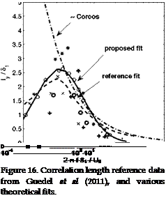
The non-dimensional plot of Fig. 16 attempts in pointing evidence of such a proportionality, but the reported data exhibit significant scatter. Determinations of both £y and di suffer from uncertainties because of ei­ther numerical or experimental resolution issues. The average theoretical

fit proposed by Guedel et al (2011) and another fit deduced from the log­normal model assuming variations of A only with the span-wise separation

are added on the figure. Both are acceptable assumptions for acoustic pre­dictions in terms of decibels. In contrast Corcos-like fitting is not, at low frequencies. Extrapolated values at high frequencies for which measure­ments cannot be achieved lead to significant differences. At 2 n f S^/Uq = 4 in Fig. 16 the new proposed fit produces 12 dB less than the other two, therefore the choice of theoretical model becomes crucial.