THE TELESCOPE MOCK-UP

The issue is to check the validity of the 13th order controller on the full 46th order plant. Uncertainties are introduced in the natural fre­quencies of the 20 bending modes contained in the identified telescope model: see chapter 2 (section 3.) for the presentation of the mock-up and chapter 4 (section 2.2) for the computation of the LFT model. A model perturbation with 20 non repeated real scalars is to be handled.

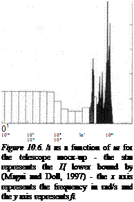
The basic algorithm of subsection 5.1 is first applied. Results are shown on Figure 10.6, which displays the fj, upper bound as a function of frequency. Note first the very fine peaks on the /і plot. An upper bound of the maximal s. s.v. over the frequency, interval [0, 1600 rad/s] is obtained as 46.80, between 1101.75 rad/s and 1103.95 rad/s. The H<i controller can thus tolerate an uncertainty of only ±2 % (и 1/46.8) in the frequencies of the bending modes. The star on Figure 10.6 corres­ponds to the Ц lower bound by (Magni and Doll, 1997), namely 44.94 at

1103.4 rad/s. The gap between the bounds is less than 4%, the result is nearly non conservative.

The associated computations were achieved in 14776s (about 4 hours) on an efficient Sun SPARCstation. If the aim is just to compute an upper bound of the maximal s. s.v., the improved algorithm of subsection 5.2 can be applied. All frequency intervals are eliminated, except the one between 1097.34 rad/s and 1114.98 rad/s. The basic algorithm is then applied to this single interval, and the same value is obtained for the upper bound of the maximal s. s.v., namely 46.80 between 1101.75 rad/s and 1103.95 rad/s. The associated computations were achieved in 3210 s (less than an hour).

50 – 45 – 40 – 35 – 30 – 25 – 20 – 15 – 10 –

5 –

For both algorithms, the computational requirement is thus not neg­ligible in the case of this example. Nevertheless, the computed value of the robustness margin is reliable, in the sense that it can be guaranteed that a critical peak on the ц plot was not missed. The result is moreover
nearly non conservative, and the telescope problem is quite challenging: the more flexible the example, the heavier the computational burden. In the case of very lightly damped flexible modes, the frequency intervals have to be chosen very small to detect very narrow and high peaks on the /г plot. In practice, the computational burden simultaneously de­pends on the structure of the model perturbation (this burden increases with the complexity of this structure – 20 real scalars in the case of this example), on the values of the damping ratios of the bending modes (roughly between 0.2 % and 2 % in the case of this example) and on the number of these bending modes (20 modes in the case of this example).