
Our heavyweight helicopter equal in the world does not have
In Rostov started production of the most load-lifting rotary-wing car The Russian holding «Helicopt[...]

Everything about aircrafts and helicopters. News and events in aviation worldwide. Civil, transportation, military helicopters and airplanes.

Everything about aircrafts and helicopters. News and events in aviation worldwide. Civil, transportation, military helicopters and airplanes.

Everything about aircrafts and helicopters. News and events in aviation worldwide. Civil, transportation, military helicopters and airplanes.

Everything about aircrafts and helicopters. News and events in aviation worldwide. Civil, transportation, military helicopters and airplanes.


In Section 2.9 we saw that flow past practical shapes of interest can be represented or simulated with suitable combination of source, sink, free vortex and uniform flow. In this section let us discuss some such flow fields.
2.10.1 Flow Past a Half-Body
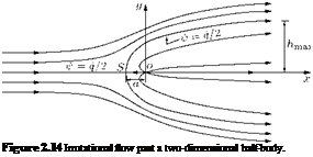 |
An interesting pattern of flow past a half-body, shown in Figure 2.14, can be obtained by combining a source and a uniform flow parallel to x-axis. By definition, a given streamline = constant) is associated
with one particular value of the stream function. Therefore, when we join the points of intersection of the radial streamlines of the source with the rectilinear streamlines of the uniform flow, the sum of magnitudes of the two stream functions will be equal to the streamline of the resulting combined flow pattern. If this procedure is repeated for a number of values of the combined stream function, the result will be a picture of the combined flow pattern.
The stream function for the flow due to the combination of a source of strength – at the origin, immersed in a uniform flow of velocity Vx, parallel to x-axis is:
f = VX r sin в + в.
2п
The streamlines of the resulting flow field will be as shown in Figure 2.14.
The streamline passing through the stagnation point S is termed the stagnation streamline. The stagnation streamline resembles a semi-ellipse. This shape is popularly known as Rankine’s half-body. The streamlines inside the semi-ellipse are due to the source and those outside the semi-ellipse are due to the uniform flow. The boundary or stagnation streamline is given by:
It is seen that S is the stagnation point where the uniform flow velocity Vx cancels the velocity of the flow from the source. The stagnation point is located at (a, n). At the stagnation point, both Vr and Ve should be zero. Thus:
![]() 1
1
Vr = – r
= Vx cos в + = 0.
2nr
This gives:
![]() –
–
2nVx’
Therefore, the stream function of the stagnation point is:
– в
fs = Vx r sin в + —.
2n
At the stagnation point S, r = a and в = n, therefore:
–
fs = Vx a sin n +——- n
2n
– – = 2.
The equation of the streamline passing through the stagnation point is obtained by setting ф = = q/2,
resulting in:
A plot of the streamlines represented by Equation (2.46) is shown in Figure 2.14. It is a semi-infinite body with a smooth nose, generally called a half-body. The stagnation streamline divides the field into a region external to the body and a region internal to it. The internal flow consists entirely of fluid emanating from the source, and the external region contains the originally uniform flow. The half-body resembles several shapes of theoretical interest, such as the front part of a bridge pier or an aerofoil. The upper half of the flow resembles the flow over a cliff or a side contour of a wide channel.
The half-width of the body is given as:
![]() q (n — в) 2 nVx
q (n — в) 2 nVx
As в ^ 0, the half-width tends to a maximum of hmax = q/(2 Vx), that is, the mass flux from the source is contained entirely within the half-body, and q = (2 hmax) Vx at a large downstream distance where the local flow velocity u = Vx.
The pressure distribution can be found from the incompressible Bernoulli’s equation:
1 2 1 2
p + 2 pu = + 2 pVx
where p and u are the local static pressure and velocity of the flow, respectively.
The pressure can be expressed through the nondimensional pressure difference called the pressure coefficient, defined as:
![]() p – Px 2 pxV.2
p – Px 2 pxV.2
where p and px are the local and freestream static pressures, respectively, px is freestream density and Vx is freestream velocity.
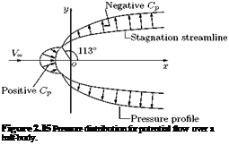 |
A plot of Cp distribution on the surface of the half-body is shown in Figure 2.15. It is seen that there is a positive pressure or compression zone near the nose of the body and the pressure becomes negative or suction, downstream of the positive pressure zone. This positive pressure zone is also called pressure-hill.
The net pressure force acting on the body can easily be shown to be zero, by integrating the pressure p acting on the surface. The half-body is obtained by the linear combination of the individual stream functions of a source and a uniform flow, as per the Rankine’s theorem which states that:
“the resulting stream function ofn potential Bows can be obtained by combining the stream functions of the individual Bows."
The half-body shown in Figure 2.15 is also referred to as Rankine’shalf-body.
![]()
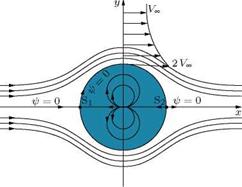
The potential function for the flow is:
![]() m
m
Ф = V^r + — cos в.
It is seen that ф = 0 for all values of в, showing that the streamline ф = 0 represents a circular cylinder of radius r = ^/m/(2nVCXl). Let r = a = ^/m/(2nVCXl). For a given velocity of the uniform flow and a given strength of the doublet, the radius a is constant. Thus, the stream function and potential function
 |
|
|
|
|
|
|
|
|
|
|
|
|
|
|
|
|
drag, is known as d’Alembert’s paradox. This discrepancy between the results of inviscid and viscous flows is because of:
• the existence of tangential stress or skin friction and
• drag due to the separation of the flow from the sides of the body and the resulting formation of wake dominated by eddies, in the case of bluff bodies, in the actual flow which is viscous.
The surface pressure in the wake of the cylinder in actual flow is lower than that predicted by irrotational or potential flow theory, resulting in a pressure drag.
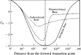
Note: For flow past a circular cylinder, there are two limits for the Cp, as shown in Figure 2.18. These two limitsare Cp = +1 and Cp = —3, at the forward and rear stagnation points (at0° and 180°, respectively), and at the top and bottom locations of the cylinder (at 90° and 270°, respectively). At this stage, it is natural to question about the validity of these limiting values of the pressure coefficient Cp for flow past geometries other than circular cylinder. Clarifying these doubts is essential from both theoretical and application points of view.
• The positive limit of +1 for Cp, at the forward stagnation point, is valid for all geometries and for both potential and viscous flow, as long as the flow speed is subsonic.
• When the flow speed becomes supersonic, there will be a shock ahead of or at the nose of a blunt-nosed and sharp-nosed bodies, respectively. Hence, there are two different speeds at the zones upstream and downstream of the shock. Therefore, the freestream static pressure and dynamic pressure
![]() to be used in the Cp relation:
to be used in the Cp relation:
![]() p – p <x>
p – p <x>
2 рП>
have two options, where p is the local static pressure. This makes the Cp at the forward stagnation point sensitive to the freestream static and dynamic pressures, used to calculate it. Therefore, Cp = +1 can not be taken as the limiting maximum of Cp, when the flow speed is supersonic.
• The limiting minimum of -3, for the Cp over the cylinder in potential flow, is valid only for circular cylinder. The negative value of Cp can take values lower than -3 for other geometries. For example, for a cambered aerofoil at an angle of incidence can have Cp as low as —6.
• Another important aspect to be noted for viscous flow is that there is no specific location for rear stagnation point on the body. The flow separates from the body and establishes a wake. The separation is taking place at two locations, above and below the horizontal axis passing through the center of the body. Also, these upper and lower separations are not taking place at fixed points, but oscillate around the separation location, because of vortex formation. Therefore, the negative pressure at the rear of the body does not assume a specified minimum at any fixed point, as in the case of potential flow. For many combinations of the geometries and flow Reynolds numbers, the negative Cp at the separated zone of the body can assume comparable magnitudes over a large portion of the wake.


