Numerical Simulation: An Example

To show the effectiveness of the DRP schemes and the radiation and outflow bound­ary conditions, the results of one special initial value problem involving all three types of disturbances will be presented below in some detail. The case under consideration consists of an acoustic pulse generated by an initial Gaussian pressure distribution at the center of the computational domain as shown in Figure 6.2. The mean flow Mach number is 0.5. Downstream of the pressure pulse, at a distance equal to one-third of the length of the computational domain, a vorticity pulse and an entropy pulse (also with Gaussian distribution) are also generated at the initial time. Since the acoustic pulse travels three times faster than the vorticity and entropy pulses in the down­stream direction, this arrangement ensures that all the three pulses reach the out­flow boundary simultaneously. In this way, it is possible to obtain a critical test of the effectiveness of the radiation as well as the outflow boundary conditions in a single simulation.

In the simulation, the variables are nondimensionalized by the following

scales:

length scale = Дх = Ду velocity scale = a0

time scale = —

a0

density scale = p0 pressure scale = p0a0.

The computational domain is divided into a 200 x 200 mesh. The initial condi­tions imposed at time t = 0 are as follows:

p = e1 exp[-a1 (x2 + y2)] 1 (acoustic pulse)

p = e1 exp[-a1 (x2 + y2)] I + e2exp[-a2((x – 67)2 + y2)] (entropy pulse)

u = e3y exp[-a3((x – 67)2 + y2)] v = – e3(x – 67) exp[-a3 ((x – 67)2 + y2)]

where e1 = 0.01, e2 = 0.001, e3 = 0.0004, a1 = (ln2)/9, a2 = a3 = (ln2)/25. The exact solution (see Tam and Webb, 1993) is.

6.4.1 Acoustic Waves

TO

u(x, y, t) = Є^2а Г/ e-^/4a1 sin(H t)J1 (Hn)H dH 10

TO

v(x, y, t) = j e-H2/4“i sin(Ht)J1 (Hn)HdH

10

TO

p(x, y, t) = p = j e-2/4a1 cos(Ht J(Hn)HdH,

10

where n = [(x – Mt)2 + y2]1/2, J1 and J0 are the Bessel functions of order 1 and 0. M is the Mach number.

6.4.2 Entropy Waves

p = u = v = 0, p = e2eTO[(x-61-Mt )2+y2].

6.4.3 Vorticity Waves

p=p=0

u(x, y, t) = e3ye-“3[(x-61-Mt)2+y2]

v(x, y, t) = – e3(x – 61 – Mt)e-аз[(x-61-Mt)2+y2].

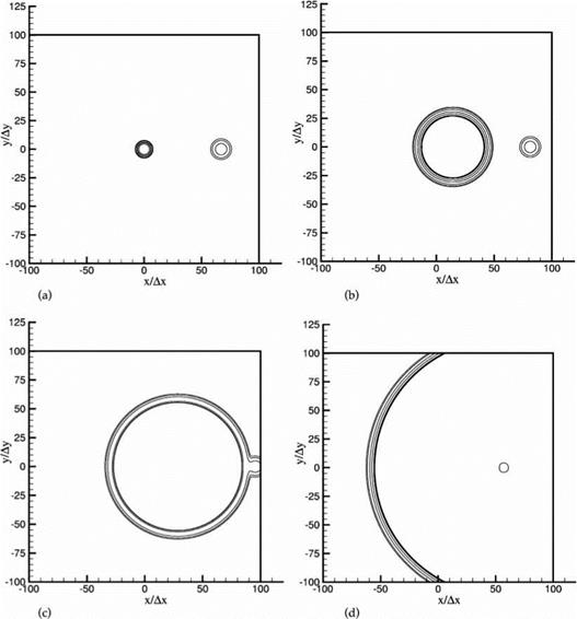
The results of the simulation will now be presented. Figure 6.3a shows the den­sity contours of the acoustic pulse at the center of the computation domain and the entropy pulse downstream at time t = 0. The vorticity pulse has no density fluctuations and, therefore, cannot be seen in this figure. Figure 6.3b shows the com­puted density contours after 500 time steps (At = 0.0569). At this time, the radius of the acoustic pulse has expanded considerably, while that of the entropy pulse remains the same. The centers of the two pulses have moved downstream by an equal

Figure 6.3. Density contours. (a) t = 0, (b) t = 500 At, (c) t = 1000 At, (d) t = 2000 At.

distance. Figure 6.3c shows the locations of the two pulses at 1000 time steps. The acoustic pulse has now caught up with the entropy pulse. At a slightly later time, the density contours of the two pulses merge and exit the outflow boundary together. Based on the 1 percent contour plot, no noticeable reflections have been observed, indicating that the outflow boundary condition is transparent. At a still later time, the acoustic pulse reaches and leaves the computation domain through the top and bottom boundaries. Again, few or no reflections can be found (to 1 percent of the incident wave amplitude). This is shown in Figure 6.3d. Finally, at 3200 time steps, the acoustic wave front reaches the inflow boundary on the left. The pulse exits the computation domain again with few observable reflections. Contours of the exact

solution are also plotted in these figures. However, the difference between the exact and numerical solution is so small, they cannot be easily seen.

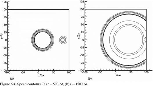
Figure 6.4a shows the contours of the magnitude of the velocity fluctuations (or speed) at 500 time steps. The center circles are those of the acoustic pulse. The circles to the right are contours associated with the vorticity pulse. The contours are constructed by interpolation between mesh points. To the accuracy allowed by this procedure, the expanding circles are, indeed, circular so that the computed acoustic wave speed is the same in all directions. Figure 6.4b gives the speed contours at 1500 time steps. At this time, the main part of the acoustic pulse has already left the outflow boundary. The vorticity pulse, having a slower velocity, has, however, not completely left the right boundary. A small piece of it can still be seen just at the outflow boundary. In this figure, the 1 percent contour exhibits some minor wiggles. A closer examination of the computed data indicates that they are generated by the graphic program and not by the simulation.

The computed density waveform along the x-axis at 500 time steps is given in Figure 6.5a. The exact solution is shown by the dotted line. The exact and computed waveforms are clearly almost identical. Figure 6.5b provides both the computed and the exact waveforms at 1000 time steps when the acoustic pulse has caught up with the entropy pulse. Again, there is good agreement between the two waveforms. Exten­sive comparisons between the computed density, pressure, and velocity waveforms with the exact solution have been carried out at different directions of propagation up to 4500 time steps when nearly all the disturbances have exited the computation domain. Good agreements are found regardless of the direction of wave propaga­tion. Such good agreements are maintained in time up to the termination of the simulation.

In addition to the simulation just described in detail, several series of simulations using more than one acoustic pulse generated at various locations of the computation

domain have been carried out. Good agreements are again found when compared with the exact solutions of the linearized Euler equations. This is true as long as the predominant part of the wave spectrum has wave numbers a and в, such that a Ax and в Ay are both less than 1.1. Overall, the results of all the simulations strongly suggest that the DRP scheme can be relied on to yield accurate results when used to simulate isotropic, nondispersive, and nondissipative acoustic, vorticity, and entropy waves. Furthermore, the scheme can be expected to reproduce the wave speeds correctly.

It is important to point out that the radiation boundary conditions (6.2) and the outflow boundary conditions (6.13) depend on the angle в. If the boundaries are far from the source, then the exact location of the source is not important. But, if the source is close to a boundary, the effectiveness of these boundary conditions would deteriorate because the direction of wave propagation is in error. An extensive series of tests involving an acoustic source put closer and closer to the boundaries have been carried out. The radiation boundary conditions appear to perform quite well even when the center of the acoustic pulse is 20 mesh points away from the boundary. The reflected wave amplitude is generally less than 2 percent of the in­cident wave amplitude. The outflow boundary conditions, on the other hand, have been observed to cause a moderate level of reflection; 15 percent for acoustic pulse initiated 20 mesh points away. This is true with or without mean flow. Recalling that the radiation and outflow boundary conditions were developed from the asymptotic solutions, the degradation of the effectiveness of the boundary conditions for sources located close to a boundary should, therefore, be expected.