LONGITUDINAL MODELS AND MODES

Assuming that the aircraft does not perform maneuvers with large excursion, it is possible to characterize the aircraft response to pitch stick inputs by considering only the lift force, drag force, and pitching moment equations.

Equation 3.22 gives the Euler angles, Equation 3.23 gives the differential equa­tions for the angular rates, and Equation 3.27 gives the polar form for V, a, and b. Assuming the aircraft to be symmetric about the XZ plane, i. e., Ixy and Iyz are zero, the general free longitudinal motion can be described by eliminating the b, p, r, and ф equations from the 6DOF state model. This leaves us with the following set of differential equations:

q cos ф — r sin ф

In the above set, although the differential equations for b, p, r, and ф are omitted from analysis, these terms still appear on the right-hand side of the equations. Measured values of b, p, r, and ф can be used to solve the above equations. Equation

5.6 can be further simplified by assuming these quantities to be small during longitudinal maneuvers and neglecting them altogether. This gives the following set of equations:

V = g( cos U sin a — sin U cos a) — — CDwind H— cos (a + sT) cos b

mm

a = — (cos U cos a + sin U sin a) + q — ~qSCL——- sin (a + sT)

V mV mV

q = Y { qScCm + T(ltx sin St + ltz cos St)}

Iy

We also know from Equation 3.30 that

Cowind = Cd cos b — Cy sin b

For small values of b

CDwind — CD

Substituting Equation 5.8 back into Equation 5.7 and assuming the thrust to be acting at CG, i. e., ltx = ltz = 0, the differential equations for longitudinal motion now take the following form:

V = g sin (U — a) — — CD + — cos (a + sT) m m a = cos (U — a) + q — ^ Cl — sin (a + St) V mV mV 1 _ q = — qScCm ly U = q

(5.9)

In the u, v, w form, the longitudinal motion of the aircraft in flight can be described by the following fourth-order model:

qS T Cx — qw — g sin U H— mm qqS — Cz + qu + g cos U m qSqc cm.

u w q U

(5.10)

y

q

where Cx, Cz, and Cm are the nondimensional aerodynamic coefficients. The above set of differential equations is commonly used to analyze aircraft longitudinal motion. This set can be further simplified, under certain assumptions, to describe the two basic oscillatory longitudinal modes (1) the heavily damped SP mode and (2) the lightly damped long period or phugoid mode. Example 5.1

The state-space equations in matrix form for LTV A-7A Corsair aircraft [4] are given as u 0.005 0.00464 —73 —31.34 u 5.63 w —0.086 —0.545 309 —7.4 w + —23.8 q — 0.00185 —0.00767 —0.395 0.00132 q —4.52 U _ 0 0 1 0 <9_ 0 At the flight condition 4.57 km (15kft) and Mach = 0.3, obtain the frequency responses for all the variables and observe the discerning effects in the dynamics. Also, obtain unit step responses for pitch rate and pitch attitude.

Solution The TFs are obtained by [num, den] = ss2tf(a, b,c, d,1); sysu = tf(num(1,:),den); sysw = tf (num(2,:),den); sysq = tf(num(3,:),den); and systheta = tf(num(4,:),den). The Bode diagrams are shown in Figure 5.1. We notice from these frequency responses that the

Bode diagram	Bode diagram
100
m TS	m TS
50
0
50	40
Frequency (rad/s)	Frequency (rad/s)
(b)
(a)
FIGURE 5.1 Frequency responses/Bode diagrams of the combined longitude modes of the LTV A-7A Corsair aircraft. (a) Forward velocity, (b) vertical velocity, (c) pitch rate, and (d) pitch attitude.

TABLE 5.1 Longitudinal Mode Characteristics of the Aircraft Eigenvalues Damping Frequency (rad/s) Mode — 1.66e-002 ± 1.39e-001i 1.18e-001 1.40e-001 Lightly damped —4.51e-001 ± 1.57e + 000i 2.76e-001 1.64e + 000 (phugoid) Relatively highly damped (short period)

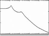
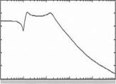
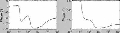
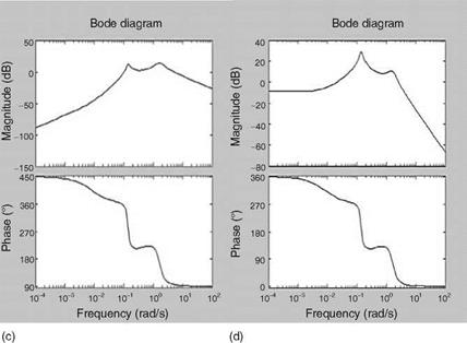
aircraft dynamics has two distinct modes: one at lower frequency and another at relatively higher frequency. This shows the feasibility of modeling these two modes separately as they are relatively well separated. One can also discern from these plots that the low- frequency mode is lightly damped compared to the higher-frequency mode, which is confirmed in Table 5.1.

In fact this shows the feasibility of separately representing the modes in two different characteristic modes, since these modes seem to be well separated. We see from Figure 5.2 that the pitch rate response is well damped and the pitch attitude response takes more time to settle. This leads to the two distinct modes discussed in the next section.