Comparison of Drag of Various Bodies

In low-speed flow past geometrically similar bodies with identical orientation and relative roughness, the drag coefficient should be a function of the Reynolds number only.

Cd = f (Re).

The Reynolds number is based upon freestream velocity V» and a characteristic length L of the body. The drag coefficient Cd could be based upon L2, but it is customary to use a characteristic area S of the body instead of L2. Thus, the drag coefficient becomes:

c _ Drag D 1PV*. S’

The factor -, in the denominator of the Cd expression, is our traditional tribute to Euler and Bernoulli. The area S is usually one of the following three types:

1. Frontal area of the body as seen from the flow stream. This is suitable for thick stubby bodies, such as spheres, cylinders, cars, missiles, projectiles, and torpedos.

2. Planform area of the body as seen from above. This is suitable for wide flat bodies such as aircraft wings and hydrofoils.

3. Wetted area. This is appropriate for surface ships and barges.

While using drag or other fluid (aerodynamic) force data, it is important to note what length and area are being used to scale the measured coefficients.

Table 2.2 gives a few data on drag, based on frontal area, of two-dimensional bodies of various cross­section, at Re > 104.

Drag coefficient of sharp-edged bodies, which have a tendency to experience flow separation regardless of the nature of boundary layer, are insensitive to Reynolds number. The elliptic cylinders, being smoothly rounded, have the “laminar-turbulent” transition effect and are therefore quite sensitive to the nature of the boundary layer (that is, laminar or turbulent).

Table 2.3 lists drag coefficients of some three-dimensional bodies. For these bodies also we can conclude that sharp edges always cause flow separation and high drag which is insensitive to Reynolds number.

Rounded bodies, such as ellipsoid, have drag which depends upon the point of separation, so that both Reynolds number and the nature of boundary layer are important. Increase of body length will generally decrease the pressure drag by making the body relatively more slender, but sooner or later the skin friction drag will catch up. For a flat-faced cylinder, the pressure drag decreases with L/d but the skin friction

2.12.1 Turbulence

Turbulent flow is usually described as flow with irregular fluctuations. In nature, most of the flows are turbulent. Turbulent flows have characteristics which are appreciably different from those of laminar flows. We have to explain all the characteristics of turbulent flow to completely describe it. Incorporat­ing all the important characteristics, the turbulence may be described as a three-dimensional, random phenomenon, exhibiting multiplicity of scales, possessing vorticity and showing very high dissipation. Turbulence is described as a three-dimensional phenomenon. This means that even in a one-dimensional flow field the turbulent fluctuations are always three-dimensional. In other words, the mean flow may be one – or two – or three-dimensional, but the turbulence is always three-dimensional. From the above discussions, it is evident that turbulence can only be described and cannot be defined.

A complete theoretical approach to turbulent flow similar to that of laminar flow is impossible because of the complexity and apparently random nature of the velocity fluctuations in a turbulent flow. Nevertheless, semi-theoretical analysis aided by limited experimental data can be carried out for turbulent flows, with instruments which have the capacity to detect high-frequency fluctuations. For flows at very low-speeds, say around 20 m/s, the frequencies encountered will be 2 to 500 Hz. Hot-wire anemometer is well suited for measurements in such flows. A typical hot-wire velocity trace of a turbulent flow is shown in Figure 2.25. Turbulent fluctuations are random, in amplitude, phase and frequency. If an instrument such as a pitot-static tube, which has a low frequency response of the order of 30 seconds, is used for the measurement of velocity, the manometer will read only a steady value, ignoring the fluctuations. This means that the turbulent flow consists of a steady velocity component which is independent of time, over which the fluctuations are superimposed, as shown in Figure 2.25(b). That is:

U(t) = U + u'(t),

U = U + u'(t)

where U (t) is the instantaneous velocity, U is the time averaged velocity, and u/(t) is the turbulent fluctuation around the mean velocity. Since U is independent of time, the time average of u'(t) should be equal to zero. That is:

t

u'(t) = 0 ; u’ = 0,

provided the time t is sufficiently large. In most of the laboratory flows, averaging over a few seconds is sufficient if the main flow is kept steady.

In the beginning of this section, we saw that the turbulence is always three-dimensional in nature even if the main flow is one-dimensional. For example, in a fully developed pipe or channel flow, as far as the mean velocity is concerned only the x-component of velocity U alone exists, whereas all the three components of turbulent fluctuations u’, v’ and w’ are always present. The intensity of the turbulent velocity fluctuations is expressed in the form of its root mean square value. That is, the velocity fluctuations are instantaneously squared, then averaged over certain period and finally square root is taken. The root mean square (RMS) value is useful in estimating the kinetic energy of fluctuations. The turbulence level for any given flow with a mean velocity U is expressed as a turbulence number n, defined as:

. /12 . /2 . /2

V u + v + w

3U

In the laboratory, turbulence can be generated in many ways. A wire-mesh placed across an air stream produces turbulence. This turbulence is known as grid turbulence. If the incoming air stream as well as the mesh size are uniform then the turbulent fluctuations behind the grid are isotropic in nature, that is, u’, v’, w’ are equal in magnitude. In addition to this, the mean velocity is the same across any cross­section perpendicular to the flow direction, that is, no shear stress exists. As the flow moves downstream the fluctuations die down due to viscous effects. Turbulence is produced in jets and wakes also. The mean velocity in these flows varies and they are known as free shear flows. Fluctuations exist up to some distance and then slowly decay. Another type of turbulent flow often encountered in practice is
the turbulent boundary layer. It is a shear flow with zero velocity at the wall. These flows maintain the turbulence level even at large distance, unlike the grid or free shear flows. In wall shear flows or boundary layer type flows, turbulence is produced periodically to counteract the decay.

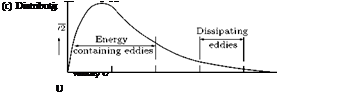
A turbulent flow may be visualized as a flow made up of eddies of various sizes. Large eddies are first formed, taking energy from the mean flow. They then break up into smaller ones in a sequential manner till they become very small. At this stage the kinetic energy gets dissipated into heat due to viscosity. Mathematically it is difficult to define an eddy in a precise manner. It represents, in a way, the frequencies involved in the fluctuations. Large eddy means low-frequency fluctuations and small eddy means high-frequency fluctuations encountered in the flow. The kinetic energy distribution at various frequencies can be represented by an energy spectrum, as shown in Figure 2.25(c).

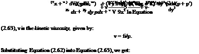
The problem of turbulence is yet to be solved completely. Different kinds of approach are employed to solve these problems. The well-known method is to write the Navier-Stokes equations for the fluctuating quantities and then average them over a period of time, substituting the following [in Navier-Stokes equations, Equation (2.23)]:

Vx = Vx + u, Vy = Vy + v’, Vz = Vz + w’

p = p + p,

where Vx, u’, Vy, v’, Vz, w’ are the mean and fluctuational velocity components along x-, y – and z-directions, respectively, and p, p’, respectively, are the mean and fluctuational components of pressure p. Bar denotes the mean values, that is, time averaged quantities.

Let us now consider the x-momentum equation [Equation (2.23)] for a two-dimensional flow:

Expanding Equation (2.64), we obtain:

In this equation, time average of the individual fluctuations is zero. But the product or square terms of the fluctuating velocity components are not zero. Taking time average of Equation (2.65), we get:

Equation (2.66) is slightly different from the laminar Navier-Stokes equation (Equation 2.63). The continuity equation for the two-dimensional flow under consideration is:

This can be expanded to result in:

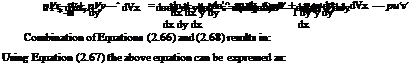
The terms involving turbulent fluctuational velocities u’ and v’ on the left-hand side of Equation (2.66) can be written as:

The terms —pul and —pu’v’ in Equation (2.69) are due to turbulence. They are popularly known as Reynolds or turbulent stresses. For a three-dimensional flow, the turbulent stress terms are pul, pv’2, pw’2, pu’v’, pv’w’ and pw’u’. Solutions of Equation (2.69) is rather cumbersome. Assumptions like eddy viscosity, mixing length are made to find a solution for this equation.

At this stage, it is important to have proper clarity about the laminar and turbulent flows. The laminar flow may be described as “ a well orderly pattern where fluid layers are assumed to slide over one another,” that is, in laminar flow the fluid moves in layers, or laminas, one layer gliding over an adjacent layer with interchange of momentum only at molecular level. Any tendencies toward instability and turbulence are damped out by viscous shear forces that resist the relative motion of adjacent fluid layers. In other words:

“laminar flow is an orderly flow in which the fluid elements move in an orderly manner such that the transverse exchange of momentum is insignificant”

and

“turbulent flow is a three-dimensional random phenomenon, exhibiting multiplicity of scales, pos­sessing vorticity and showing very high dissipation. ”

Turbulent flow is basically an irregular flow. Turbulent flow has very erratic motion of fluid particles, with a violent transverse exchange of momentum.

The laminar flow, though possesses irregular molecular motions, is macroscopically a well-ordered flow. But in the case of turbulent flow, there is the effect of a small but macroscopic fluctuating velocity superimposed on a well-ordered flow. A graph of velocity versus time at a given position in a pipe flow would appear as shown in Figure 2.26(a), for laminar flow, and as shown in Figure 2.26(b), for turbulent flow. In Figure 2.26(b) for turbulent flow, an average velocity denoted as V has been indicated. Because this average is constant with time, the flow has been designated as steady. An unsteady turbulent flow may prevail when the average velocity field changes with time, as shown in Figure 2.26(c).