Reflection of Acoustic Waves by a Plane Wall

A detailed analytical analysis of the reflection of acoustic waves from a wall (see Figure 6.8) using the solid wall boundary conditions described above has been carried out by Tam and Dong (1994). Their analysis clearly shows that, in addition to the reflected acoustic wave, spurious waves (parasite waves) are reflected off the wall. Furthermore, spatially damped numerical waves of the computation scheme are also excited at the wall boundary. These waves form a numerical boundary layer. Space limitations would not allow a discussion of the analytical part of their work. However, their numerical results are useful to provide an assessment of the accuracy and quality of solution in adopting the ghost point method to enforce wall boundary conditions.

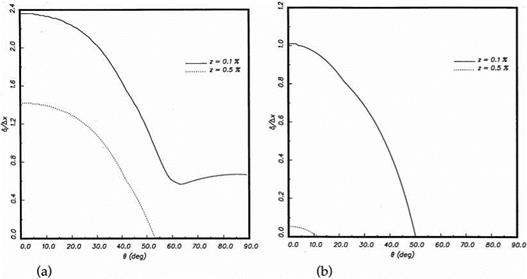
Suppose numerical boundary layer thickness, 8z, is defined to be the distance between the wall and where the spurious numerical wave solution drops to z times the magnitude of the reflected acoustic wave amplitude, e. g., 50 005 denotes the boundary

layer thickness based on 0.5 percent of the reflected wave amplitude. Figure 6.9a shows the calculated numerical boundary layer thickness as a function of the angle of incidence when a spatial resolution of X/Ax = 6 (Ay = Ax) is used for computing the acoustic waves; X is the wavelength. Two thicknesses are shown, one corresponds to z = 0.005 (0.5 percent), the other z = 0.001 (0.1 percent). This figure indicates that the numerical boundary layer is thickest for normal incidence. In this case 50 001 is almost equal to 2.5 Ax. Figure 6.9b shows the corresponding numerical boundary layer thickness if a spatial resolution of X/Ax = 10 is used in the computation. It is clear that with better spatial resolution the numerical boundary layer thickness decreases.

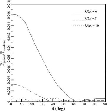
Figure 6.10 shows the dependence of the magnitude of the reflected parasite wave (grid-to-grid oscillations), |pparasite/PincidentI, on the angle of incidence for dif­ferent spatial resolution. At X/Ax = 6, the reflected parasite wave can be as large as more than 1 percent of the incident wave amplitude at normal incidence. At glazing incidence, i. e., beyond в = 50°, there is generally very little parasite wave reflected off the wall. The magnitude of the reflected parasite wave would be greatly reduced if the spatial resolution in the computation is increased. By using 10 or more mesh points per acoustic wavelength in the computation, the reflected parasite wave is so weak that they may be ignored entirely.

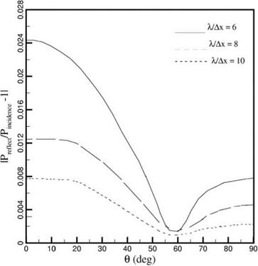
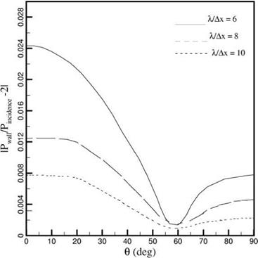
Figure 6.11 is a plot of the deviation from perfect acoustic reflection. It is a measure of the quality of the numerical solid wall boundary condition. For perfect reflection, the ratio of the reflected wave amplitude to that of the incident wave, IPreflected/PincidentI, is unity. Figure 6.11 shows that, by using the proposed numerical solid wall boundary condition, the deviation from perfect reflection is small. It is of the order of 1 percent even when only 6 mesh points per acoustic wavelength are used in the computation. When acoustic waves impinge on a wall, the pressure at the wall is twice the incident sound pressure. This phenomenon is usually referred to as pressure doubling. Figure 6.12 shows that the computed wall pressure would,

indeed, be close to twice the incident sound pressure level for X/Ax = 6. Again, when a better spatial resolution is used in the computation, e. g., X/Ax = 8, the computed results would better reproduce the pressure-doubling phenomenon.