Our heavyweight helicopter equal in the world does not have
In Rostov started production of the most load-lifting rotary-wing car The Russian holding «Helicopt[...]

Everything about aircrafts and helicopters. News and events in aviation worldwide. Civil, transportation, military helicopters and airplanes.

Everything about aircrafts and helicopters. News and events in aviation worldwide. Civil, transportation, military helicopters and airplanes.

Everything about aircrafts and helicopters. News and events in aviation worldwide. Civil, transportation, military helicopters and airplanes.

Everything about aircrafts and helicopters. News and events in aviation worldwide. Civil, transportation, military helicopters and airplanes.


The SP is a relatively well-damped, high-frequency oscillation mode. Chapter 7 shows some typical time history plots of longitudinal SP motion. The amplitude ratio
|
FIGURE 5.2 Unit step responses for pitch rate (—) and pitch attitude (—) of the longitude modes of the LTV A-7A Corsair aircraft. |
Since a « w, Equation 5.14 can also be written in terms of a instead of w:
a= – a + f1 + Zq)q + Zde 8e u0 u0 u0
q = Maa + Mqq + Mde 8e
|
![]() Z
Z
Zw = —; Mw
uo
Putting the SP two degrees of freedom model in state-space form x = Ax + Bu and neglecting Zq
The characteristic equation of the form (AI – A) for the above system will be
A2 — (m9 + —)a + (/MqZa — мЛ = 0 (5.17)
uo uo
Solving for the eigenvalues of the characteristic equation yields the following frequency and damping ratio for the SP mode:
Example 5.2
The aerodynamic derivatives determined from flight test conducted with 3-2-1-1 pilot stick command input for a transport aircraft are given as
Zq = -0.0085, Za = -0.480, Zq = Q.1Q2, ZSe = 0.652,
MQ = 0.472, Ma = -4.916, Mq = -1.946, Mde = -7.011
The Z-force derivatives are assumed to be normalized with longitudinal velocity component uQ.
Write an appropriate mathematical model and obtain TF and frequency response of the SP model.
Solution
Based on the derivatives given we can build the following longitudinal SP model:
a = Zq + Zaa + (1 + Zq)q + Zge 8,
q = M0 + Maa + Mqq + M8e 8e
The state-space form is given as
|
a |
-0.482 (1 + 0.102) |
a |
|
|
q. |
-4.916 – 1.946 |
q |
The TFs are obtained as [numsp, densp] = ss2t/(a, b,c, d,1) and sysalpha = t/(numsp(1,:), densp) and sysq = t/(numsp(2,:),densp). The bias/‘‘nought’’ derivatives are ignored. The two TFs are
a(s) 0.652s – 6.457 d q(s) -7.011s – 6.585
d(sj = s2 + 2.428s + 6.355 ™ d(s) = s2 + 2.428s + 6.355
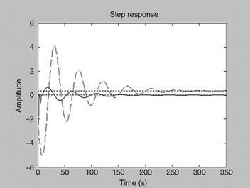
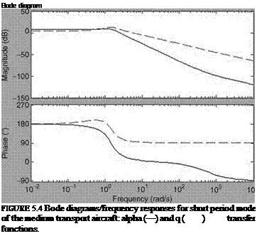
The SP frequency and damping ratio are obtained as: [spfreq, spzeta] = damp (sysalpha) = [2.521 rad/s, 0.4816]. The frequency/Bode diagrams are shown in Figure 5.3. Thus, we see the distinct SP mode, though for a different aircraft.
Example 5.3
The aerodynamic derivatives for an air force medium transport aircraft are given as
Za/U0 = -0.66, ZSe/щ = 0.01, Ma = -1.74, Mq = -0.67, MSe = -5.33
Write an appropriate mathematical model and obtain TFs and frequency responses of the SP model. Also, obtain the unit step responses.
Solution
Based on the derivatives given we can build the following longitudinal SP model:
a = (Za/u0)a + q + (ZSe/uq )8e q — Maa + Mqq + Mge 8e
The state-space form is given as
|
a |
—0.66 |
1 |
a |
‘ 0.01 ‘ |
||
|
q. |
— |
— 1.74 |
—0.67 |
q |
+ |
—5.33 |
The TFs are obtained as [num, den] — ss2t/(a, b,c, d,1) and sysalpha — t/(num(1,:),den) and sysq — t/(num(2,:),den). The two TFs are
a(s) 0.01s – 5.323 , q(s) -5.33s – 3.535
and
Se(s) s2 + 1.33s + 2.182 8e(s) s2 + 1.22s + 2.182
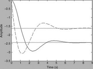
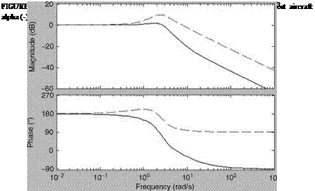
The SP frequency and damping ratio are obtained as [spfreq, spzeta] — damp(sysalpha) — [1.48 rad/s, 0.45]. The frequency/Bode diagrams are shown in Figure 5.4. The unit step responses are shown in Figure 5.5.
![]()
|