Transition to Turbulence

In most practical aerodynamic applications, the boundary-layer flow is predomi­nantly turbulent. We consider laminar flows in detail to appreciate the role of vis­cosity in a fluid flow, as well as to establish definitions and ideas in a simple-flow case. Also, for a distance downstream of an airfoil or wing leading edge, the bound ary layer is laminar. However, the laminar boundary layer soon goes through a compli­cated series of changes, after which a turbulent boundary layer emerges. A turbulent­boundary-layer flow exhibits unsteady, chaotic motion that has a random character and that contains large-scale eddies. The series of changes within the boundary layer that convert a laminar to a turbulent boundary layer usually occur over a finite dis­tance, called a transition region. Because of the major differences in laminar and turbulent skin friction (and heat transfer), it is desirable to be able to predict (or estimate) both the start and the end of the transition region. Much experimental and analytical/numerical effort has been expended in this regard. We limit our discussion to an overview of the transition process from a physical perspective, with estimates of the streamwise extent of the transition region.

Recall that a laminar boundary layer in a steady flow consists of flow in smooth, steady laminas. However, the laminar shear layer is subject to small disturbances that occur in any flow (e. g., surface vibration, noise, freestream turbulence, surface imperfections, or roughness). These external disturbances usually are infinitesimal and random. They act as forcing functions that trigger two-dimensional wave-like disturbances within the laminar boundary layer. These waves, which travel down­stream in the boundary layer, are called Tollmein-Shlichting waves (T-S waves), named after two researchers who conducted basic studies on the stability of these disturbance waves in the early 1930s.

Below a certain minimum Re number, these T-S waves damp out. This number is called the critical Reynolds number, which usually is based on a boundary-layer – thickness dimension, such as 5*, rather than a streamwise dimension, x. For a
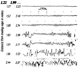
flat-plate boundary layer, Recrit, 5* typically has a value of about 700, corresponding to a value of Recr, x of about 165,000. Values of Re numbers used in this discussion, of necessity, must be prefaced by “about” or “approximately” because they depend so strongly on the environment (e. g., freestream turbulence level) of a particular boundary layer. This is not the transition point; it simply represents the lowest value of the Re number at which small disturbances in the boundary layer can be ampli­fied. For the remainder of the discussion, we think of holding the flow velocity and properties constant and increasing the Re number by increasing the downstream distance, x, from the plate leading edge. At a value above the critical Re number, the disturbance waves within a certain frequency band are found to amplify with downstream distance. Linear-stability theory is used to predict the frequency band and the rate of amplification. A classical series of measurements was made by Schu – bauer and Skramstad in the 1940s that confirmed this amplification of the T-S waves (See discussion in Schlichting, 2003). Local velocities were measured in a flat-plate boundary layer with a fast-response instrument called a hot-wire anemometer; the results are shown in Fig. 8.29. Notice that at about 5 ft. (1.52 m), wave amplification is evident; at 6 ft. (1.83 m), the local flow is becoming nonlinear; and at 8 ft. (2.44 m), it is fully turbulent.

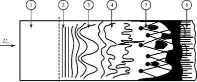
As the T-S waves are amplified, a complicated three-dimensional struc­ture evolves. The waves begin to exhibit spanwise variations, and distorted vortex structures appear. Turbulent spots are formed, which are small regions of intense velocity fluctuations. These spots grow in size and number, finally coalescing into a fully turbulent boundary layer. The process of boundary-layer transition is shown in Fig. 8.30 (White, 1974).

Figure 8.29. Oscillograms showing natural transition from laminar to turbulent flow (See discussion in Schlichting, 2003).

О I—► x Rcrit

Figure 8.30. Schematic of the transition process on a flat plate (White).

The transition Re number, Retrx, is the value of the Re number at which the boundary layer becomes fully turbulent. For a smooth flat plate with a low – turbulence level in the external flow, this value can be as large as (about) Retrx = 1 x 107. This value must be used with caution. For example, the boundary layer on a swept wing becomes turbulent much closer to the leading edge than for a straight wing (or flat plate) due to three-dimensional effects. Looking at Fig. 8.29, note that the caption states that this experimental result, as well as the value for Retr, x quoted previously, is for “natural” transition (i. e., transition of a boundary layer in the pres­ence of minimal outside disturbances). At times, it is desirable to force transition to a more upstream location (i. e., smaller value of x). For example, consider the wind-tunnel test of a model wing that is conducted to predict the behavior of a much larger full-scale wing at the same velocity. On the full-scale wing, the turbu­lent boundary layer may be established close to the leading edge; whereas on the model, the same transition Re number (i. e., the same x-dimension) corresponds to a chordwise distance much closer to the trailing edge. Recall from a previous discussion that the location of the boundary-layer separation point is sensitive to whether the boundary layer is laminar or turbulent. Thus, wind-tunnel tests at high angles of attack may be misleading because the boundary-layer separation point can not be located correctly. In such a case, the boundary layer on the model often is “tripped” (i. e., forced transition) by gluing a roughness strip (e. g., sandpaper) to the model wing surface in a spanwise direction a short distance downstream of the leading edge. Such a comparatively large disturbance causes a turbulent boun­dary layer to be established much closer to the leading edge than in the natural – transition case. Care must be taken that the artificial disturbance introduced is not so large as to lead to a badly distorted (hence, unrealistic) turbulent boundary-layer profile downstream.

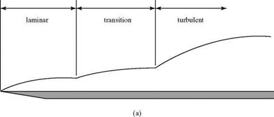
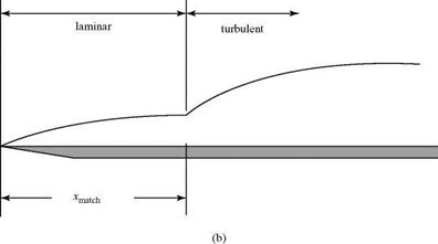
Figure 8.31. Actual and assumed boundary-layer growth.

If we want to calculate simply the behavior of an entire boundary layer from laminar through turbulent, the details in the transition region must be avoided. This normally is accomplished by making an assumption about the behavior of tran­sition. The actual boundary layer, containing a transition region, is like that shown in Fig. 8.31a. For purposes of calculation, it is assumed that the boundary layer is first laminar and then turbulent, as shown in Fig. 8.31b; the change occurs instantly at some Re number value. In similarity analyses, a virtual origin for the turbulent boundary layer may be found by matching 5* or 0 for the two boundary layers at Rematchx (i. e., at %match) . In numerical analyses, the downstream matching calcu­lation is switched from laminar-to-turbulent defining equations at xmatch. The value of Rematchx is somewhat arbitrary and comes from experience. Because it must be larger than Recrit, a typical value of Rematch used is several hundred thousand.

The following factors stabilize a laminar boundary layer and thus delay tran­sition in an incompressible flow:

1. Favorable streamwise pressure gradient. Laminar-flow airfoils are specially shaped so as to maintain a chordwise favorable pressure gradient over the air­foil for as long as possible. Boundary layers stabilized in this way are said to have natural laminar flow (NLF).

2. Suction. Bleeding off the laminar boundary layer from a wing surface through spanwise suction slots or through porous surfaces stabilizes the laminar boundary layer. The suction inhibits boundary-layer growth and also alters the boundary-layer profile, which affects stability characteristics. Designs that use an artificial mechanism such as suction to maintain a laminar boundary layer are said to have laminar flow control (LFC).

3. Cooling the surface. Cooling a surface increases the value of Recrit

4. Making the surface smoother. Increasing surface roughness has a destabilizing effect on a laminar boundary layer.

5. Decreasing the turbulence level in thefreestream. This applies to wind-tunnel tests. Turbulence in the atmosphere has a negligible effect on the transition of a boun­dary layer on a flight vehicle. However, the freestream turbulence level in a wind – tunnel test section has a major influence on transition because it acts as a trigger for boundary-layer disturbance waves. We must be careful when comparing detailed boundary-layer turbulence measurements taken in different wind tunnels.

A good discussion of transition is in White, 1986, and a detailed review of tran­sitional boundary layers is provided in, Lauchle, 1991. A comprehensive review of flow control and control devices is found in Gad-El-Hak, 1989.

The increasing cost of jet fuel has made the subject of transition and LFC increas­ingly important. Holmes et al. found that for a high-performance business jet operating at Mcruise = 0.7, NLF on the wings, fuselage, and engine nacelles leads to a drag reduc­tion of 24 percent of total airplane drag (Holmes et al., 1988). Further information on full-scale and wind-tunnel tests on NLF surfaces is found in Holmes et al., 1984.

For design purposes (see Raymer, 1989), a typical conventional aircraft (i. e., no special boundary-layer treatment) may be considered to have laminar flow over perhaps 10 to 20 percent of the wings and tails and virtually no laminar flow over the fuselage. With some NFC incorporated into the design, laminar flow can extend over as much as 50 percent of the wings and tails and about 20 to 35 percent of the fuselage. Thus, any discussion of incompressible boundary layers is incomplete without treating the turbulent boundary layer, which is the topic of the next section.