Our heavyweight helicopter equal in the world does not have
In Rostov started production of the most load-lifting rotary-wing car The Russian holding «Helicopt[...]

Everything about aircrafts and helicopters. News and events in aviation worldwide. Civil, transportation, military helicopters and airplanes.

Everything about aircrafts and helicopters. News and events in aviation worldwide. Civil, transportation, military helicopters and airplanes.

Everything about aircrafts and helicopters. News and events in aviation worldwide. Civil, transportation, military helicopters and airplanes.

Everything about aircrafts and helicopters. News and events in aviation worldwide. Civil, transportation, military helicopters and airplanes.


By analysis of his carefully conducted series of smoke-injection tests, Landgrebe [9] reduced the results to formulae giving the radial and axial coordinates of a tip vortex in terms of azimuth angle, with corresponding formulae for the inner sheet. From these established vortex positions (the so-called prescribed wake) the induced velocities at the rotor plane may be calculated. The method belongs in a general category of prescribed-wake analysis, as do earlier analyses by Prandtl, Goldstein and Theodorsen, descriptions of which are given by
|
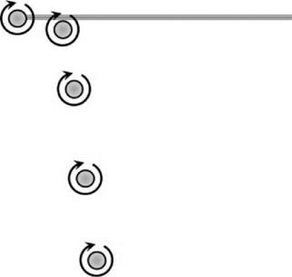
Figure 2.27 Schematic of vortex motion |
Bramwell. These earlier forms treated either a uniform vortex sheet as pictured in Figure 2.25 or the tip vortex in isolation, and so for practical application are effectively superseded by Landgrebe’s method.
More recently, considerable emphasis has been placed on free-wake analysis, in which modern numerical methods are used to perform iterative calculations between the induced – velocity distribution and the wake geometry, both being allowed to vary until mutual
|
|
|
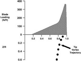
Figure 2.29 Wake sheet and tip vortex trajectory |
consistency is achieved. This form of analysis has been described for example by Clark and Leiper [10]. Generally the computing requirements are very heavy, so considerable research effort also goes into devising simplified free-wake models which will reduce the computing load. The computing power available is consistently increasing with time; however, the complexity of the methods always seems to fill the available computing capability.
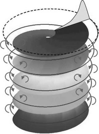
Calculations for a rotor involve adding together calculations for the separate blades. Generally this is satisfactory up to a depth of wake corresponding to at least two rotor revolutions. A factor which helps this situation is the effect on the tip vortex of the upwash ahead of the succeeding blade – analogous to the upwash ahead of a fixed wing. The closer the spacing between blades, the stronger the effect from a succeeding blade on the tip vortex of the blade ahead of it; thus it is observed that when the number of blades is large, the tip vortex remains approximately in the plane of the rotor until the succeeding blade arrives, when it is convected downwards. In the ‘far’ wake, that is beyond a depth corresponding to two rotor revolutions, it is sufficient to represent the vorticity in simplified fashion; for example, free – wake calculations can be simplified by using a succession of vortex rings, the spacing of which
is determined by the number of blades and the mean local induced velocity. Eventually in practice both the tip vortices and the inner sheets from different blades interact and the ultimate wake moves downwards in a confused manner.
There we leave this brief description of the real wake of a hovering rotor and the methods used to represent it. This branch of the subject is often referred to as vortex theory. It will be touched on again in the context of the rotor in forward flight (Chapter 5). For more detailed accounts, the reader is referred to the standard textbooks and the more specific references which have been given in these past two sections.