Our heavyweight helicopter equal in the world does not have
In Rostov started production of the most load-lifting rotary-wing car The Russian holding «Helicopt[...]

Everything about aircrafts and helicopters. News and events in aviation worldwide. Civil, transportation, military helicopters and airplanes.

Everything about aircrafts and helicopters. News and events in aviation worldwide. Civil, transportation, military helicopters and airplanes.

Everything about aircrafts and helicopters. News and events in aviation worldwide. Civil, transportation, military helicopters and airplanes.

Everything about aircrafts and helicopters. News and events in aviation worldwide. Civil, transportation, military helicopters and airplanes.


Equations for the induced velocities in hover were derived using the momentum method. A variation of the same method applies to forward flight and starts with the same equation:
T = m/sec x Av
In order to define the mass flow and the change in velocity, it is helpful to go back to the aerodynamics of a wing for an analogy. When a wing generates lift, at least in theory, it affects all the air, both near and far. Of course, the air adjacent to the
wing is affected the most, whereas at large distances from the wing the effect is negligible. It may be shown that for an ideal wing with an elliptical lift distribution, the downward acceleration of the total mass of air is mathematically equivalent to uniformly accelerating only the mass of air in a round stream tube whose diameter is equal to the wing span. This purely mathematical coincidence should not be given a physical connotation. For the wing shown in Figure 3.2, the momentum equation may be written:
|
|
|
|
|
|
 |
For most forward flight conditions, it may be assumed that vl is small compared with V, so that:
, aTPP will always be assumed to be small enough that: cos сц-рр = 1.
Using this definition, another alternative form for the induced velocity equation is:
SIR CT
p =————-
H 2
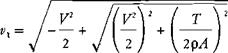
These equations apply to conditions where the forward velocity is relatively large with respect to the induced velocity. It is sometimes necessary to make calculations at low speeds, where this assumption is not valid. For these cases, the momentum equation is:
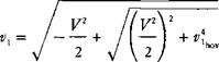
T=f>Ay/V2 + vl 2v, Solving this without making any assumptions gives:
|
|
or:
|
|
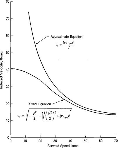
A comparison of the results of using this equation and the simpler one derived earlier is shown in Figure 3.3, where vx in ft/sec is plotted against forward speed in knots for the example helicopter. It may be seen that for the example helicopter, the two equations give essentially the same results above about 30 knots.
The simple equation for induced velocity derived here is known as the constant momentum induced velocity. A more realistic view sees the induced velocity as the result of a very complex vorticity pattern, consisting of trailing, shed, and bound vortex elements associated with the lift and the change of lift on each blade element. This complexity is of great importance when studying blade loads and helicopter vibration, but it has been found that for most performance calculations the use of the constant momentum value—which represents the average of the complex velocity field—gives reasonably accurate results. There are, however, two helicopter trim problems that require modifications to the simple theory. The first of these is the calculation of the effects of the rotor wake impinging on a horizontal stabilizer in low-speed forward flight. In hover, the average dynamic pressure in the fully developed wake is equal to the disc loading. Experience has shown, however, that local dynamic pressures in the wake in hover and forward flight may be significantly higher than this. Some feeling for this may be obtained by studying the plots of the wake dynamic pressure below a hovering rotor, which were shown in Figure 1.19 of Chapter 1. Test results reported in reference 3.1 show that the download pressure to which a horizontal stabilizer may be subjected in low-speed flight can be as much as three times the main rotor disc loading. Assuming a drag coefficient of 2 for the stabilizer in this condition gives a dynamic
|
FIGURE 3.3 Induced Velocities in Low-Speed Flight for Example Helicopter |
pfessure in the wake of 1.5 times the disc loading. This can be the source of disconcerting trim shifts in transition flight.
Another analysis problem that will be examined in detail later is that of calculating the lateral blade flapping in forward flight. For this, it has been found necessary to represent the local induced velocity at the disc as:
v=vA 1 + К — cos w I * /
where j/ is the blade azimuth position, being zero over the tail. This equation defines an induced velocity distribution that is small at the leading edge of the disc and large at the trailing edge, as shown in Figure 3.4. Smoke studies of the induced velocities around wind tunnel models of rotors in forward flight reported in references 3.2 and 3.3 show that the average velocity distribution does indeed have
 |
this general pattern and, furthermore, that the induced flow at the leading edge of the disc is essentially zero. This observation leads to assigning the distortion factor, К, a value of unity, so that:
This applies to relatively high speeds—say above 100 knots—but at low speeds, the distortion may be somewhat higher. This is shown in Figure 3.5, taken from reference 3.4, which reports on flight tests and wind tunnel experience on the very rigid rotor Sikorsky Advancing Blade Concept helicopter. From the cyclic pitch required to trim, the distortion factor in the induced velocity equation could be determined. The figure indicates that while a value of unity may be good for high speeds, in the transition region it may be as high as 2.
Several alternative forms of this equation are discussed in reference 3.5, a study of the surprisingly large lateral flapping that occurs at low speeds.. A more rigorous derivation of the induced velocity distribution using vortex theory is given in reference 3.6.