
Our heavyweight helicopter equal in the world does not have
In Rostov started production of the most load-lifting rotary-wing car The Russian holding «Helicopt[...]

Everything about aircrafts and helicopters. News and events in aviation worldwide. Civil, transportation, military helicopters and airplanes.

Everything about aircrafts and helicopters. News and events in aviation worldwide. Civil, transportation, military helicopters and airplanes.

Everything about aircrafts and helicopters. News and events in aviation worldwide. Civil, transportation, military helicopters and airplanes.

Everything about aircrafts and helicopters. News and events in aviation worldwide. Civil, transportation, military helicopters and airplanes.


It has already been emphasized that linearization of EOMs can be carried out only if the small perturbation assumption is not violated. The same is true in the case of a missile, i. e., the linearity constraint can be invoked if the changes in the incidence angles and angular body rates are small. To design a control system for a missile, the procedure is to define an operating point (in terms of Mach and altitude) and consider the aerodynamic derivatives pertaining to the operating point to remain unchanged within a small region of the selected flight condition. The control system is then designed to meet the specific requirements of system phase lag, damping, and bandwidth. In this manner, several test conditions are investigated. Detailed analysis is carried out by also considering the configuration changes due to change in mass and shift in CG as the fuel gets consumed. From Equations 3.34 and 3.35, neglecting the gravity terms and considering only the Y-force, Z-force, and the equations for angular accelerations, the control equations for the missile can be expressed as [5]
~ = v + rU = Yvv + Yrr + ~Sr 8r Z = w — qU = Zww + Zqq + Zde 8e p = Lpp + LSa 8a (5.31)
q = Mww + Mqq + Ml8e 8e Г = Nvv + Nrr + Ndr 8r
where ~ and Z denote the specific forces (accelerations) given by
Z = Y/m Z = Z/m
and ~v, ~r, ~8 , Zw, …, N8 are specific derivatives. Full values of these derivatives can be computed given the information on mass and inertia characteristics of the missile.
The aileron deflection in a missile is given by one of the following formulae:
4 (81 + 82 + 83 + 84); 1 (81 + 83); 1 (82 + 84)
If only two surfaces act in differential mode, we have elevator deflection: 1 (81 — 82); and rudder deflection: 1 (82 — 84).
A very useful concept in control system design is that of TF. A TF gives the relationship between the output and input to a system and is defined as the ratio of the Laplace transform of output to the Laplace transform of input. Some of the aerodynamic TFs obtained by taking Laplace of Equation 5.31 are given below [5]:
(a) Roll rate/aileron (p/Sa)
Consider the p equation in Equation 5.31. Taking Laplace, we have
sp — Lpp = LSa 8 a
or
![]() P _ LSg _ L8g jLp
P _ LSg _ L8g jLp
8 a S — Lp 1 + ts
The above aerodynamic TF gives steady-state gain equal to —L8 /Lp and time constant t equal to — 1/Lp.
(b) Lateral acceleration/rudder (Y /8r)
Simplifying Y and r equations in Equation 5.31 by eliminating r and v and neglecting the ~r derivative which is generally very small, we obtain the following expression for TF for YY 8r:
![]() £ = s2 YSr — sNrYSr + U(N~8г – N8г~у) 8r = s2 — s(Nr + ~v) + (UNV + Nr ~v)
£ = s2 YSr — sNrYSr + U(N~8г – N8г~у) 8r = s2 — s(Nr + ~v) + (UNV + Nr ~v)
If шп denotes the undamped natural frequency and § denotes the damping ratio, for the TF given in Equation 5.33, we have
u>2n = UNv + Nr ~v and 2§w„ = Nr + ~v
In the expression for the term UNv is generally much larger than NrYv. In Equation 5.33, the steady-state gain is given by i70^^8r2^8^v).
(c) Yaw rate/rudder (r/8r)
Once again, the TF for r/8r can be obtained by eliminating v from Y and r equations in Equation 5.31. This yields
![]() r sNSr + (Ny Y8r NSr Yv)
r sNSr + (Ny Y8r NSr Yv)
8r = s2 — s(Nr + Yv) + (UNv + Nr Yv)
Comparing Equations 5.33 and 5.34, one observes that шп and § are the same for both TFs.
(d) Sideslip/rudder (b/8r)
Eliminating r from Y and r equations in Equation 5.31 and, for small incidence angles, assuming b = v/U, TF for b /8r can be expressed as
|
|
|
|
![]()
Once again, the vn and § for the above TF is the same as that for TFs expressed in Equations 5.33 and 5.34.
Example 5.7
For a surface-to-air missile with rear controls the yaw aerodynamic derivatives for a certain flight condition (Mach = 1.4, H = 1.5 km, and U = 467 m/s) [5] are given as
Yv = -2.74; Vv = 0.309; Ys = 197; Ns = -534; Vr = -2.89
The other details are length = 2 m, mass = 53 kg, and moment of inertia = 13.8 kg m2. The missile latex (lateral acceleration) rudder control TF is given as
fly(s) Yss2 – YsNrs – U(NSYV – NVYS)
d(s) _ s2 – (Yv + Nr)s + YvNr + UNv
With the values given obtain the missile TF, its characteristic modes, frequency responses, and step input responses.
Solution
The following TF is obtained:
ay(s) 197s2 + 569.33s – 467(1463.16 – 60.87)
Й(?Г _ s2 + 5.63s + (7.92 + 144.3)
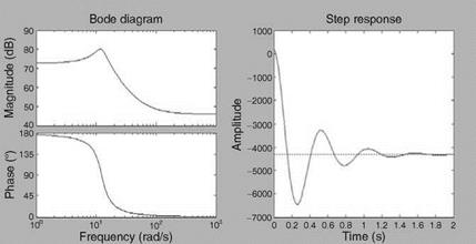 |
The latex dynamic mode is second-order oscillatory: -2.815 ± 12.0123i; the natural frequency is 12.3 rad/s; and the damping ratio is 0.228. The frequency response and the unit step rudder response for the latex are shown in Figure 5.9.
