Our heavyweight helicopter equal in the world does not have
In Rostov started production of the most load-lifting rotary-wing car The Russian holding «Helicopt[...]

Everything about aircrafts and helicopters. News and events in aviation worldwide. Civil, transportation, military helicopters and airplanes.

Everything about aircrafts and helicopters. News and events in aviation worldwide. Civil, transportation, military helicopters and airplanes.

Everything about aircrafts and helicopters. News and events in aviation worldwide. Civil, transportation, military helicopters and airplanes.

Everything about aircrafts and helicopters. News and events in aviation worldwide. Civil, transportation, military helicopters and airplanes.


3.1 Basic Method
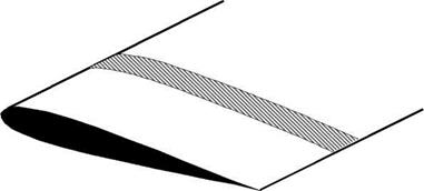
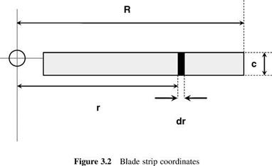
Blade element theory is basically the application of the standard process of aerofoil theory to the rotating blade. A typical aerodynamic strip is shown in Figure 3.1 and the appropriate notation for a typical strip is shown in Figure 3.2. Although in reality flexible, a rotor blade is assumed throughout to be rigid, the justification for this lying in the fact that at normal rotation speeds the outward centrifugal force is the largest force acting on a blade and, in effect, is sufficient to hold the blade in rigid form. In vertical flight, including hover, the main complication is the need to integrate the elementary forces along the blade span. Offsetting this, useful simplification occurs because the blade incidence and induced flow angles are normally small enough to allow small-angle approximations to be made.
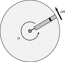
Figure 3.3 is a plan view of the rotor disc, seen from above. Blade rotation is anticlockwise (the normal system in the UK and the USA) with angular velocity Q. The blade radius is R, the tip speed therefore being QR, alternatively written as VT. An elementary blade section is taken at radius r, of chord length c and spanwise width dr. Forces on the blade section are shown in Figure 3.4. The flow seen by the section has velocity components Qr in the disc plane and (VC + Vi) perpendicular to it. The resultant of these is:
The blade pitch angle, determined by the pilot’s collective control setting (see Chapter 4), is У. The angle between the flow direction and the plane of rotation, known as the inflow angle, is f, given by:
Basic Helicopter Aerodynamics, Third Edition. John Seddon and Simon Newman. © 2011 John Wiley & Sons, Ltd. Published 2011 by John Wiley & Sons, Ltd.
|
|
|
Figure 3.1 General strip used in blade aerodynamic calculations
|
|
Figure 3.3 Rotor disc viewed from above |
 |
|
or for small angles, which we shall assume:
The angle of incidence of the blade section, denoted by a, is seen to be:
![]()
![]() a = 0—ф
a = 0—ф
The elementary lift and drag forces on the section are:
dL = 2 p U2 • c dr • CL
dD = pU2 • c dr • CD
Resolving these normal and parallel to the disc plane gives an element of thrust:
dT = dL cos ф—dD sin ф (3.6)
and an element of blade torque:
dQ = (dL sin ф + dD cos f)r (3.7)
The inflow angle ф may generally be assumed to be small; from Equation 3.3 this may be questionable near the blade root where Or is small, but there the blade loads are themselves small also. Masking the reasonable assumption that the rotor blade section has a high lift/drag
ratio, the following approximations can therefore be made:
U ‘ Or
dT ‘ dL (3.8)
dQ ‘ (f dL + dD)r
|
0 _ _ , о _ (VC + Vi) _ ^ /ri л лЛ 1 — mZD — mZ + 1 — OR — xf (3.14) 1 is known as the inflow factor. Now the element of thrust becomes, noting that we have N blades: |
 |
It is convenient to introduce dimensionless quantities at this stage. We write:
which leads to:
![]() dCT = sCLx2 dx
dCT = sCLx2 dx
Integrating along the blade span gives the rotor thrust coefficient as:
The rotor power requirement is given by:
![]() P = OQ
P = OQ
 |
||
Note that the power coefficient is defined as:
Hence CP and Cq are identical in value (essentially there is a O term multiplying both the numerator and denominator).
The definitions used in this book contain a half in the denominator. This is not universal as some analyses omit the half. It is also apparent that the normalizing factors are based, as in the lift coefficient, on a dynamic pressure and a reference area. The thrust, torque and power coefficients use the disc area. However, the introduction of blade element theory (BET) gives equations which feature the blade area, so another set of coefficients can be defined to reflect this:
T T Ct
2r(OR)2 • NcR 1 r(OR)2 • A •(NcR/A) s
![]() Q_________________ Q__________ =Cq
Q_________________ Q__________ =Cq
2r(OR)2 • R • NcR 2r(or)2 • r • a • (NcR/A) s
P P________ Cp
1 r(OR)3 • NcR 1 r(OR)3 • A •(NcR/A) s
These are related to the original coefficients via the rotor solidity.
To evaluate Equations 3.18 and3.21 it is necessary to know the spanwise variation ofblade incidence a and to have blade section data which give Cl and Cd as functions of a. The equations can then be integrated numerically. Since a is given by (в — ф), its distribution depends upon the variations of в, the blade pitch, and (VC + V), the total induced velocity, represented by the inflow factor l. Useful approximations can be made, however, which allow analytical solutions with, in most cases, only small loss of accuracy.