Modeling of Highly Swept Leading – Edge Separation
The modeling of leading-edge separation from highly swept wings is somewhat simpler than the modeling of the unswept leading-edge separation. The primary reason is that in this case the vorticity generated at the leading edge is immediately conveyed downstream by the chordwise flow and since there is no vorticity accumulation near the leading edge there is no time-dependent wake shedding (as in the unswept leading-edge case). Modeling is possible if the basic information about the location of the flow separation line and the strength of the separated shear layer is supplied to the potential-flow solution. Usually such information is generated by a local viscous solution, experiments, or even by using some parameters obtained from the potential-flow solution. For example, when modeling the flow over low aspect ratio delta wings with sharp leading edges, the location of the separation line is fixed along the sharp leading edge (recall that a sharper leading edge results in a stronger L. E. vortex and more vortex lift, Fig. 14.45). In regard to specifying the strength of the leading-edge shear layer (leading-edge wake), two of the more frequently used possibilities are:
1. Estimate vortex strength by using Eq. (14.15), which requires the calculation of the velocity above and under the wake. In this case the effect of leading-edge radius can be included in the К coefficient such that К = 0.6 for a sharp leading edge and some smaller values of К may be used as the leading-edge radius increases.
2. The second approach, which is simpler and seems to yield reasonable results in the range of a= 10-35°, is the treatment of the L. E. wake as a regular wake. The strength of the wake panel adjacent to the wake (Fig. 14.53) is then calculated by a “Kutta condition” as in Eq. (9.15):
Hw = t*u-I*L (14.20)
where ци and juL are the corresponding upper and lower surface doublet strengths along the separation line (see also Fig. 13.37).
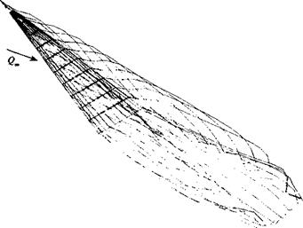
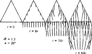
The shape of the separated wake can be calculated by the methods presented in Section 14.1 and in the following examples the calculations are based on the time-stepping method14 37,14 38,12 13 (which is based on the unsteady flow formulation of Chapter 13). The wake rollup is obtained by gradually releasing vortex wake panels from the sharp L. E., similarly to the wake-shedding process at the trailing edge, until the fully developed wake shape is obtained. This is shown schematically in Fig. 14.54 for several time steps and for simplicity only the longitudinal vortex lines are shown (but the wake is constructed by using vortex rings, as shown in Fig. 14.53). The vortex rollup is determined by the momentary velocity induced by the wing and its wakes (as described in Section 13.12, Eqs. (13.153) and (13.154)). Results for
FIGURE 14.53
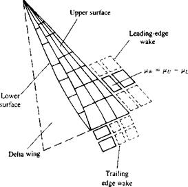 Vortex ring (or constant-strength doublet) model for both trailing and leading edge wakes shed from slender delta wings.
the lift curve of this delta wing (based on this model) are presented in Fig. 14.55. At the lower angles of attack (less than —10°), the lift curve slope is well predicted by the linear formulation of R. T. Jones (Eq. (8.94)) (CL = (л/2Ж«)). At higher incidences, however, the leading-edge vortices increase the lift, as indicated by a sample of experimental results (Refs. 14.39-14.41). This vortex lift is not predicted by the basic linear panel method (using only the trailing-edge wake) since the leading-edge wake and its vortex lift is not included. The addition of the separated L. E. vortex model (shown in Fig. 14.56) increases the wing’s lift and improves the comparison with the experimental data. At very high angles of attack (above 40°), however, vortex breakdown results in the wing’s lift loss, a condition that is not modeled here.
![]()
|
|
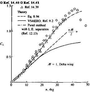 FIGURE 14.55
Comparison between experimental and calculated lift coefficient for a slender delta wing (using a panel method1213 with leading – edge vortex model).
|
|
|
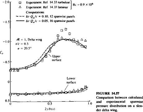
The spanwise pressure distribution at the x/c = 0.5 station is presented in Fig. 14.57. The wing model consists of 248 panels with 12 spanwise equally spaced panels, and the nondimensional time step is 0.1 chord (Qa„ At/с = 0.1). Results for a denser computation grid (328 panels, 16 spanwise panels, 6» A tic = 0.05) are shown by the solid line, and both computations show the suction peaks due to the leading-edge vortices. The experimental results with the turbulent boundary layer of Ref. 14.33 (Ле = 0.9х 106 for both experiments) indicate a secondary vortex near the leading edge that was not modeled here. In general, it was found that the lift of the delta wing was less sensitive to
|
FIGURE 14.58 Vortex wake lines behind a slender delta wing moving forward in a coning motion. |
 |
 |
a coarser grid and larger time steps than the pressure distribution over the wing’s surface. In cases when computer time saving is considered and larger time steps are applied, the spanwise pressure distribution will smear, but the lift will change by only a few percent.
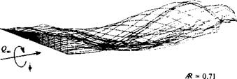
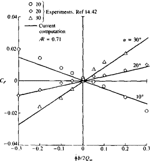
For a demonstration of more complex motions, the wake lines behind a delta wing with an aspect ratio of 0.71, undergoing a coning motion, are presented in Fig. 14.58. The wing angle of attack a was set relative to the x, y, z frame of reference (pitching along x/c = 0.6), and then the wing was rotated about the x axis at the rate <f>. Computed rolling moments are compared with the experimental data of Ref. 14.42 in Fig. 14.59. The slopes of the computed rolling moment curves, which change rapidly with variations of angle of attack, compare reasonably well with the experiments. For angles of attack higher than 30° and for roll rates <j>b/2Q<„ larger than 0.1, vortex breakdown bends the experimental curves and larger differences between the experiment and the computations are detected.


