Angle of Attack of the Blade Element

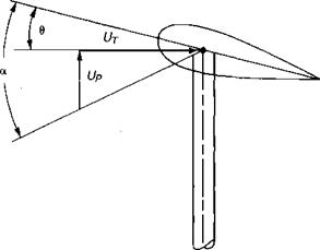
In order to define increments of lift and drag acting on a blade element in forward flight, it is necessary to write the equation for the angle of attack at the element as a function of the radial station and the azimuth position. For this analysis, it will be assumed that the rotor has no hinge offset and that flapping harmonics above the first may be neglected. The local angle of attack, shown in Figure 3.28, is made up of two angles just as it is in hover—the blade pitch and the inflow angle:

a = 0 + tan-1

4

The use of UT in this equation is based on the concept originally proved fdr swept wing airplanes—that only the velocity normal to the leading edge counts. The blade pitch has already been defined as a Fourier series:

f

9 = 0O + 0X — — Л, cosxj/ — Bx sin j/

К

and the equation for the tangential velocity, UT, has been derived:

UT = CtR I + |i sin у

The perpendicular velocity, Up, is a vector that is perpendicular to the blade quarter-chord line and lies in a plane that contains the rotor shaft. It is positive going up and consists of several components, as shown in Figure 3.29.

FIGURE 3.28 Angle of Attack at Blade Element

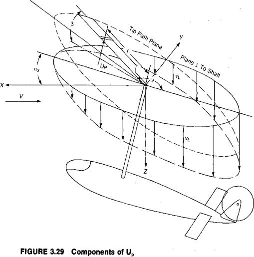
Up = Vas — vL — rp — Fp cos |/

A description of these components follows:

• F a—the component of forward speed that is parallel to the rotor shaft. (Note that a positive angle of attack is with the nose up, as shown in Figure 3.29, just as it is for airplanes. Helicopters generally fly nose down, or with negative angles of attack, but the sign convention was established when only autogiros—which do fly nose up—had rotors.)

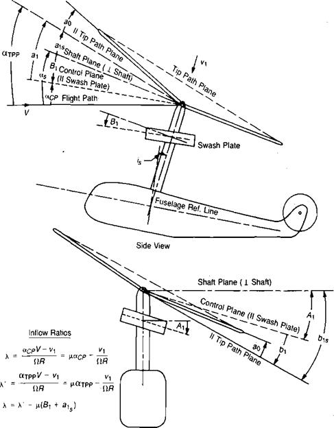
• Vp—the local induced velocity, which for normal flight conditions may be considered to be parallel to the rotor shaft: For subsequent analysis, it will be convenient to use the angle of attack of the tip path plane as a reference angle rather than the angle of attack of the plane perpendicular to the shaft. Figure 3.30 shows the relationships between the various planes which are used in rotor analyses. Much of the early work, such as in references 3.16 and 3.17, used the control plane as a basic reference system. This is sometimes called the "plane of no feathering.” Later investigators for convenience have switched to the shaft plane or to the tip path plane—which is the "plane of no flapping”—as their basic reference planes. From Figure 3.30, it may be seen that:

Ct; ~ ^TPP ~ ais

Rear View

FIGURE 3.30 Rotor Angle Relationships

If all angles—including un~l(vJflR)—are expressed in degrees, then a is also in degrees. Note that when a is expressed in this form, the combinations of cyclic pitch and flapping, (Al — bj and (Bt + atJ, occur as primary variables. This is a consequence of the equivalence of flapping and feathering, which says that as far as rotor aerodynamics are concerned, one degree of cyclic pitch produces the same effect as one degree of flapping. (This equivalence strictly applies only to rotors with zero flapping hinge offset, but it is a good assumption for the analysis of performance of rotors that have moderate flapping hinge offsets or even for hingeless rotors which flap through structural bending. For analysis of stability and control, the hinge offset is significant and is discussed in Chapter 7.) In some of the early rotor analyses, such as in reference 3.17, these combinations of cyclic pitch and flapping are referred to as flapping with respect to the "plane of no feathering” and are designated ax and bx

a — + as

K = -(Ax-bx)

The equation for the local angle of attack contains several types of quantities that are either known or which may be computed: [3]

• |i, tip speed ratio = V/ClR.

• 0-rpp, angle of attack of the tip path plane required to put rotor thrust, helicopter weight, and helicopter drag into equilibrium.

• a0, coning of blades, which is established by equilibrium between lift and centrifugal forces.

• vJClR, induced velocity ratio, where vx is from momentum equation.

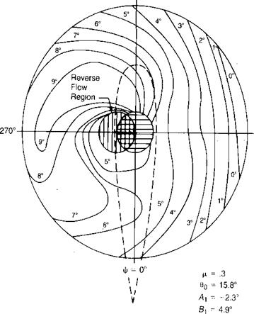
The flight conditions for the example helicopter have been determined at a tip speed ratio of 0.3 (115 knots) by methods to be outlined later, and the resultant angle of attack distribution has been plotted in Figure 3.31. Note that the angle of attack of the advancing tip is in the neighborhood of 0°, while the retreating tip is nearly 10°. The angle of attack on each side of the boundary of the reverse flow region goes to ± 90°, but since the local velocity is zero along this boundary, these high angles have little practical significance.

Ф = 180° otjpp – -3.7° Cjla = .086

CLOSED-FORM EQUATIONS

Again, just as in hover, there are two schemes for integrating the forces on the blade elements to give rotor performance. The first method involves performing the integration of the equations mathematically to produce closed-form equations as a function of rotor geometry and flight conditions. The second method, suitable for a computer, performs the integrations by numerical methods. The closed-form integration method produces equations that are useful for rough calculations and for giving an understanding of the important factors; but since it must use simplifying assumptions in order to make the integration feasible, accuracy is sacrificed for convenience. The numerical integration method, which will be outlined later, uses a minimum of assumptions so that the resulting accuracy is high, but it is inconvenient without investing considerable time and effort in programming and checking out the computer.