Closed-Form Integration for Thrust

Just as in hover, the rotor thrust in forward flight can be computed from the integration of the lift on each blade element along the blade and around the azimuth. The same equation for the incremental lift applies:

A L = qctcAr

or in terms of blade element conditions:

AL = – UladcAr 2

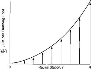
where both the velocity, UT, and the angle of attack, a, have been derived as functions of r/R and of j/. The integration procedure is simple in principle but tedious in application because of the large number of terms involved. For this reason, the method will be outlined in general, but detailed steps will be left to the ambitious student. The integration starts with the equation of lift per running foot:

AL p tt2

a — acUr Ct Ar 2

For a given value of j/, the lift per running foot is as shown in Figure 3.32. The lift on the blade is designated as Lh and is the area under the curve.

* A L

Lift Distribution along Blade

Lift Distribution Around Azimuth FIGURE 3*32 Illustration of Integration for Thrust

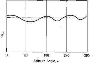
For each value of j/, the integral can be evaluated and the result plotted as a function of \l, as in Figure 3.32. The average lift per blade, Lb, around the azimuth is the area under the curve divided by the length of the horizontal axis which is 360° or 2n radians:

L>/4

Substituting for Ly the average lift per blade becomes a double integral on r and J/. The total thrust is equal to the number of blades times the average lift per blade:

In

this stage of the analysis and discussed later along with the effect of the reversed flow region.)

The integration is straightforward and may be done using tables of integrals. The result is:

The term, СЦ-рр — (Bl + <*!), is the angle of attack of the swashplate or control plane with respect to the flight path, as shown in Figure 3.30. In classical treatments of rotor aerodynamics, such as in references 3.16 and 3.17, the flow perpendicular to this control plane is called the inflow:

Inflow = F[aTPP — (B, + )] — vy

and normalizing by dividing by tip speed gives the inflow ratio, X:

X=(l[aTPP – (B, + at)]~ vJClR

or in terms of shaft angle:

X=i[a,-BA-vJdR

As a function of 0, |i, and X, the thrust coefficient is:

This form is convenient when working with flapping rotors without cyclic pitch such as tail rotors or the rotors of simple autogiros. It is, however, somewhat awkward to use for the analysis of helicopters with cyclic pitch, since the value of

rotors, a more convenient equation results from using the angle of attack of the tip path plane as a basic parameter, rather than the angle of attack of the control plane. This is obtained by using the equation for the sum of longitudinal cyclic pitch and longitudinal rotor flapping, (Bx + ax), which is derived by writing the equation for the aerodynamic rolling moment on the disc and then equating it to zero since the rotor must be trimmed aerodynamically with respect to rolling moments. The increment of rolling moment is:

AR = —ALr sin j/

and the total rolling moment is:

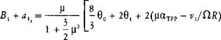When this equation is expanded in terms of UT and a, equated to zero, and then solved for (Bx + dj), the result is:

In this equation, the inflow term is with respect to the tip path plane and will be designated A/:

X’ = |iaTpp – vJClR

[Note that A.’ = A.+ n(B1 + dlj).] Thus:

Using this in the equation for X and performing the algebra gives a new equation for CT/o as a function of 0, |i, and X’.

The new inflow ratio, V, can be evaluated easily from known flight conditions. The angle of attack of the tip path plane is:

(Df + HM + HT) (G. W. – Le)

Methods for evaluating the main and tail rotor H-forces and the fuselage lift in forward flight will be discussed later, but since they are generally small, it may be assumed that for a first approximation:

or

Tivirad

A CT/o

. From the momentum equation previously derived:

vJClR — Ct/g 2^

Thus X’ can be evaluated for a first approximation from the flight conditions and the helicopter configuration:

X’