Modelling helicopter flight dynamics: building a simulation model

It is beyond dispute that the observed behaviour of aircraft is so complex and puzzling that, without a well developed theory, the subject could not be treated intelligently. Theory has at least three useful functions;

a) it provides a background for the analysis ofactual occurrences,

b) it provides a rational basis for the planning of experiments and tests, thus securing economy ofeffort,

c) it helps the designer to design intelligently.

Theory, however, is never complete, final or exact. Like design and con­struction it is continually developing and adapting itself to circumstances.

(Duncan 1952)

3.1 Introduction and Scope

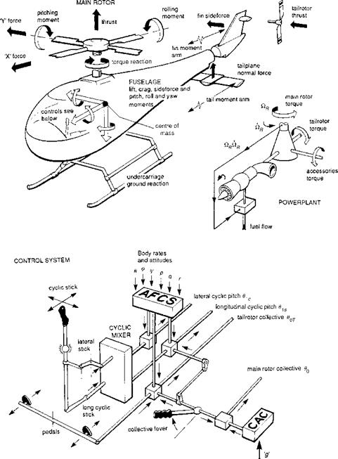
The attributes of theory described by Duncan in this chapter’s guiding quote have a ring of eternal validity to them. With today’s perspective we could add a little more. Theory helps the flying qualities engineer to gain a deep understanding of the behaviour of flight and the limiting conditions imposed by the demands of flying tasks, hence providing insight and stimulating inspiration. The classic text by Duncan (Ref. 3.1) was directed at fixed-wing aircraft, of course. Describing the flight behaviour of the helicopter presents an even more difficult challenge to mathematical modelling. The vehicle can be viewed as a complex arrangement of interacting subsystems, shown in component form in Fig. 3.1. The problem is dominated by the rotor and this will be reflected by the attention given to this component in the present chapter. The rotor blades bend and twist under the influence of unsteady and nonlinear aerodynamic loads, which are themselves a function of the blade motion. Figure 3.2 illustrates this aeroelastic problem as a feedback system. The two feedback loops provide incidence perturbations due to blade (and fuselage) motion and downwash, which are added to those due to atmospheric disturbances and blade pitch control inputs. The calculation of these two incidence perturbations dominates rotor modelling and hence features large in this chapter. For the calculation of aerodynamic loads, we shall be concerned with the blade motion relative to the air and hence the motion of the hub and fuselage as well as the motion of the blades relative to the hub. Relative motion will be a recurring theme in this chapter, which brings into focus the need for common reference frames. This subject is given separate treatment in the appendix to this chapter, where the various axes transformations required to derive the relative motion are set down. Expressions for the accelerations of the fuselage centre of gravity and a rotor blade element are

Fig. 3.1 The helicopter as an arrangement of interacting subsystems

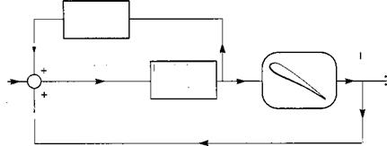
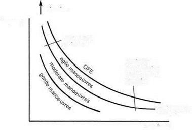Fig. 3.2 Rotor blade aeroelasticity as a feedback problem

derived in the Appendix, Sections 3A.1 and 3A.4, respectively. Rotor blades operate in their own wake and that of their neighbour blades. Modelling these effects has probably consumed more research effort in the rotary-wing field than any other topic, ranging from simple momentum theory (Ref. 3.2) to three-dimensional flowfield solutions of the viscous fluid equations (Ref. 3.3).

The modelling requirements of blade motion and rotor downwash or inflow need to be related to the application. The terms downwash and inflow are used synony­mously in this book; in some references the inflow includes components of free stream flow relative to the rotor, and not just the self-induced downwash. The rule of thumb, highlighted in Chapter 2, that models should be as simple as possible needs to be borne in mind. We refer back to Fig. 2.14 in the Introductory Tour, reproduced here in modified form (Fig. 3.3), to highlight the key dimensions – frequency and amplitude. In flight dynamics, a heuristic rule of thumb, which we shall work with, states that the

vibrabon

frequency

rotor modes aclivatcd

non Imeat aerodynamics and Etmclural dynamics

equi-rssponse contour

amplitude

modelled frequency range in terms of forces and moments needs to extend to two or three times the range at which normal pilot and control system activity occurs. If we are solely concerned with the response to pilot control inputs for normal (correspond­ing to gentle to moderate actions) frequencies up to about 4 rad/s, then achievement of accuracy out to about 10 rad/s is probably good enough. With high gain feedback control systems that will be operating up to this latter frequency, modelling out to 25-30 rad/s may be required. The principal reason for this extended range stems from the fact that not only the controlled modes are of interest, but also the uncontrolled modes, associated with the rotors, actuators and transmission system, that could poten­tially lose stability in the striving to achieve high performance in the primary control loops. The required range will depend on a number of detailed factors, and some of these will emerge as we examine model fidelity in this and the later chapters. With respect to amplitude, the need to model gross manoeuvres defines the problem; in other words, the horizontal axis in Fig. 3.3 extends outwards to the boundary of the operational flight envelope (OFE).

It is convenient to describe the different degrees of rotor complexity in three levels, differentiated by the different application areas, as shown in Table 3.1.

Appended to the fuselage and drive system, basic Level 1 modelling defines the conventional six degree of freedom (DoF) flight mechanics formulation for the fuse­lage, with the quasi-steady rotor taking up its new position relative to the fuselage instantaneously. We have also included in this level the rotor DoFs in so-called multi­blade coordinate form (see Section 3.2.1), whereby the rotor dynamics are consolidated as a disc with coning and tilting freedoms. Perhaps the strongest distinguishing feature of Level 1 models is the analytically integrated aerodynamic loads giving closed form

Table 3.1 Levels of rotor mathematical modelling Level 1 Level 2 Level 3 Aerodynamics linear 2-D dynamic inflow/local momentum theory analytically integrated loads nonlinear (limited 3-D) dynamic inflow/local momentum theory local effects of blade vortex interaction unsteady 2-D compressibility numerically integrated loads nonlinear 3-D full wake analysis (free or prescribed) unsteady 2-D compressibility numerically integrated loads Dynamics rigid blades (1) quasi-steady motion (2) 3 DoF flap (3) 6 DoF flap + lag (4) 6 DoF flap + lag + quasi-steady torsion (1) rigid blades with options as in Level 1 (2) limited number of blade elastic modes detailed structural representation as elastic modes or finite elements Applications parametric trends for flying qualities and performance studies well within operational flight envelope low bandwidth control parametric trends for flying qualities and performance studies up to operational flight envelope medium bandwidth appropriate to high gain active flight control rotor design rotor limit loads prediction vibration analysis rotor stability analysis up to safe flight envelope

expressions for the hub forces and moments. The aerodynamic downwash representa­tion in our Level 1 models extends from simple momentum to dynamic inflow.

The analysis of flight dynamics problems through modelling is deferred until Chapters 4 and 5. Chapter 3 deals with model building. For the most part, the model elements are derived from approximations that allow analytic formulations. In this sense, the modelling is far from state of the art, compared with current standards of simulation modelling. This is particularly true regarding the rotor aerodynamics, but the so-called Level 1 modelling described in this chapter is aimed at describing the key features of helicopter flight and the important trends in behaviour with varying design parameters. In many cases, the simplified analytic modelling approximates reality to within 20%, and while this would be clearly inadequate for design purposes, it is ideal for establishing fundamental principles and trends.

There are three sections following. In Section 3.2, expressions for the forces and moments acting on the various components of the helicopter are derived; the main rotor, tail rotor, fuselage and empennage, powerplant and flight control system are initially considered in isolation, as far as this is possible. In Section 3.3, the combined forces and moments on these elements are assembled with the inertial and gravitational forces to form the overall helicopter equations of motion.

Section 3.4 of this chapter takes the reader briefly beyond the realms of Level 1 modelling to the more detailed and higher fidelity blade element and aeroelastic rotor formulations and the complexities of interactional aerodynamic modelling. The flight regimes where this, Level 2, modelling is required are discussed, and results of the kind of influence that aeroelasticity and detailed wake modelling have on flight dynamics are presented.

This chapter has an appendix concerned with defining the motion of the aircraft and rotor in terms of different axes systems as frames of reference. Section 3A.1 de­scribes the inertial motion of an aircraft as a rigid body free to move in three translational and three rotational DoFs. Sections 3A.2 and 3A.3 develop supporting results for the orientation of the aircraft and the components of the gravitational force. Sections 3A.4 and 3A.5 focus on the rotor dynamics, deriving expressions for the acceleration and velocity of a blade element and discussing different axes systems used in the literature for describing the blade motion.