Error equations for terrestrial navigator

10.2.4.4 . The terrestrial navi­gation system uses as its main reference the local geographic frame. Although it is an inertial instrument and subject to Newton’s equations, it emphasizes the local – level plane. In gimbaled systems the platform with its accelerometers is torqued to

INS Error Equation Tilt Equation Gravitational Error

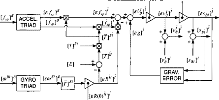
Fig. 10.27 Implementation of the error equations of the space-stabilized INS.

remain level, as the vehicle proceeds over the curved Earth. Double integration of the specific force renders the ground distance. For strap-down systems the onboard computer maintains the direction cosine matrix. Although the accelerometers are mounted on the vehicle, the conversion to local-level coordinates is readily made through this transformation.

Because many of the six-DoF simulations are based on the flat-Earth assumption, the terrestrial navigator is particularly well suited for this approach. The inertial frame becomes the Earth frame and the inertial coordinate system the local-level axes. However, recall that the local-level plane is not just the local tangent, but the curved surface of the Earth unwrapped into a plane. To account for this effect, we introduce the coupling of the tilt to the velocity error via the Earth’s radius.

The INS error equation (10.92), already derived for the inertial-referenced INS, is now based on the Earth E as an inertial reference and the local level coordinate system ]L, as computed by the INS processor:

L

= mBi[£/sp]B – [sRtE]L[T]BL[fp]B + [sg]L (10.95)

The tilt equation (10.93) receives an additional term because the tilt error of a terrestrial navigator grows now also as a result of the velocity error

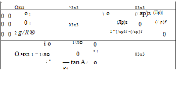
Note in particular that the second component of the velocity error couples into the third tilt component through the term (tan a//?®), which is a function of the vehicle’s latitude a. We attribute gravitational errors only to altitude uncertainties (ssbi)b and neglect other effects. The change in magnitude of the gravitational acceleration is then based on Newton’s gravitational attraction

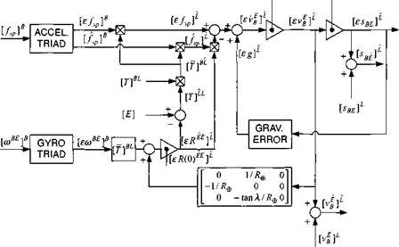
With these provisions we can modify the inertial-referenced INS of Fig. 10.27 and draw the schematic of the terrestrial navigator in Fig. 10.28. The Earth frame has become the inertial frame, and the computed inertial coordinates are replaced by the computed local-level coordinates. Notice the additional leveling loop that introduces the uncertainty in the calculation of the tilt rotation tensor [eT?££]L. The main output variables are the computed values of position [іВ£і£, velocity [rB]£, and the direction cosine matrix [T]BL. They are needed as input to seeker and guidance models, as well as parameters for plotting trajectory traces. You can find an implementation of the terrestrial INS in the CADAC SRAAM6 and SRAAM5 simulations, Module S4. It is suitable for both pseudo-five – and six-DoF simulations in conjunction with the Hat-Earth assumption.

The error term in Fig. 10.28 can also be reduced to a linear state variable formulation if we drop the term of the specific force perturbations [£/sp]B in Eq. (10.95) and reverse the vector product of the tilt skew-symmetric tensor with the specific force. Introducing the error components

£S 1	■ K£]l =	£1>1		єф
£S2	£1>1	. [r££]£ =	єв
Є S3		£1>1		єф

[ev(0)ff [е*(0)в£]2 Fig. 10.28 Implementation of the error equations of the terrestrial stabilized INS.

popularized by Widnall and Grundy 8:

eij

£S 2 es3

£l)[

ev2

£V3

єф

ев

єф

(10.98)

These are nine first-order, linear differential equations, exhibiting the two major error couplings of local-level INS systems. The tilt vector couples with the specific force into the velocity derivative channel and the velocity vector couples with the Earth’s radius into the tilt derivative channel. The gravitational coupling occurs in the vertical channel between the altitude error and the vertical velocity derivative.

I found these equations particularly useful for Kalman-filter studies. To suppress errors, Kalman filters use navigation sensors to correct INS uncertainties. Embed­ded in the filter is a dynamic model of the INS error growth. In a typical simulation the actual error growth is modeled by Eqs. (10.95-10.97), while the Kalman fil­ter mimics this process with the simplified state model of Eq. (10.98). If you are interested in pursuing this topic, refer to the excellent references by Maybeck21
or Stengel.22 As an example, the CADAC CRUISE5 simulation, Modules SI, S3, and S4 illustrate the modeling and integration of a Kalman filter between sensor measurements and INS. Although written for a five-DoF application, the code is equally pertinent for six-DoF models. To follow the code, however, a sound foundation in filtering is a prerequisite.

As a final topic, 1 need to address the proper initialization of INS errors. In the real world the transfer alignment process initializes the INS. Any imperfections cause initial uncertainties of the nine states of position, velocity, and tilt. Similar uncertainties should initialize the error equations in the simulation. The transfer alignment errors are known stochastically by their covariance matrix Po, a 9 x 9 matrix of the variances and covariances of the nine-state vector єхо. For a particular simulation run we have to extract an initial error vector from the Gaussian distribution, represented by this covariance matrix.

The Cholesky decomposition will help us in this process by taking the square root of the covariance matrix у/Pq (you can use the subroutine MATCHO in the CADAC UTL3.FOR file). Combining it with a random Gaussian (9×1) vector, having unit standard deviation gauss, yields the initial INS error state

*0 = sfPo gauss (10.99)

A word of caution is appropriate at this point. The initial covariance matrix is not diagonal because the transfer alignment process intentionally couples states to reduce instrument and initialization errors. Therefore, a realistic simulation should not be initialized by stochastically independent states, but by correlated errors, as represented by a covariance matrix with off-diagonal covariances.

The modeling of INS is an important part of a high-fidelity six-DoF simulations. After staying with me through this much-abbreviated tour, you should understand the error equations that are found in the CADAC simulation examples. Perhaps you have even gained a general appreciation for the modeling of INS systems. However, to become better rooted in this subject, you should study in detail the recommended references.