Turbulence
Atmospheric turbulence is air movement on a small scale. It is caused by the instabilities of pressure and temperature distributions in clouds, near the ground, and in the wind-shear regions of the jet stream. The fluctuations are time and space dependent. Because we cannot predict with certainty the behavior of the air molecules, we use statistical descriptors like standard deviation and power spectral density to classify the severity and spectral characteristics of turbulence.
For simulation purposes we make four assumptions that will ease the modeling task. The statistical properties of the turbulence are stationary (independent of time), homogeneous (independent of location in space), isotropic (independent of direction), and larger than the airplane (all parts of the airplane are equally affected). Two statistical representations are in good agreement with measurements: the von Karman29 and Dryden30 models. Although both yield similar results, the Dryden spectrum is preferable because it is easier to implement in simulations.
I will keep the modeling task simple. We limit ourselves to the one-dimensional Dryden spectrum and superimpose its turbulence on the air mass in the load factor plane of the aircraft or missile. (The load factor plane contains the total incidence angle a’). I pick this plane because our main interest is in the variability of the incidence angle and its effect on the vehicle.
Figure 10.46 shows the total incidence angle a’ as it relates to the angle of attack a and sideslip angle f3. We already encountered this spherical triangle in Fig. 3.19 with the corresponding angular relationship of Eq. (3.24). The aeroballistic wind axes A and 3A, which contain also the B body axis are embedded in the load factor plane. The transformation matrix [T]AB is given by Eq. (3.19).
Our goal is to express the movement of the turbulent air particles T wrt to the steady air mass A by the velocity vector vA and coordinate it in geographic axes [vA]G. The turbulence component r normal to the vehicle’s velocity vector v# in the load factor plane is expressed in the aeroballistic wind coordinates
[n^]A = [0 0 r]
With the two TMs [TAB and [T]BG we obtain the desired form
[vA]G = [T]bg[T]ab[va]A (10.140)
The entire movement of the turbulent air v B wrt Earth consists of the turbulence vA and the steady wind velocity v B. We program this superposition in geographic
|
coordinates
[^]G = K]C + [^]C 00.141)
In Eq. (10.139) we used v^G as wind vector. If we want to include turbulence, we supplement it by [Vj]G and obtain the expanded expression
K]B = mBC{k£]c – (kA]c + Kf)} (10.142)
The vehicle’s velocity wrt air is now dependent on the geographic velocity Vg, the turbulent wind Vj, and the steady wind Уд.
Now we turn to the task of generating the velocity traces r based on the onedimensional Dryden turbulence model. First, we need to convert the spatial penetration of turbulent air into a temporal process. Figure 10.47 shows an aircraft with velocity V preparing to fly into a turbulence field with sine-type vertical velocity distribution of length L. The spatial frequency of the wave is £2 = Ът/L. It takes an aircraft the time T — L/V to traverse the wave. The aircraft experiences the wave with the temporal frequency ш — 2л/T = 2л/(L/V).
Turbulent air consists not just of waves of one frequency but of a whole spectrum. Their spectral density is modeled by Dryden’s function, expressed in the nondimensional frequency m — шТ — a>L/V
![]()
![]() a2 L 1 + Зпт2
a2 L 1 + Зпт2
2л V (1 + ти2)2
 |
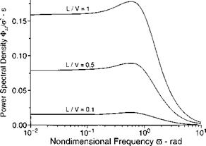
where a is the standard deviation of the turbulence in meters/second. The Dryden power spectral density function is shown in Fig. 10.48 for three L/V ratios. They
|
Fig. 10.49 Correlation length of turbulence. |
peak near m = 0.6. For an aircraft traveling at V = 300 m/s and a turbulence correlation length L — 150 m, the peak frequency occurs at o> = 1.2 rad/s, not far removed from the pitch frequency of a large aircraft.
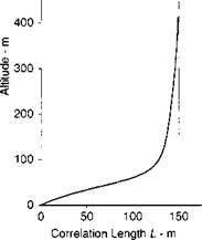
Correlation length L and standard deviation a are obtained from atmospheric measurements. Lumley and Panowsky31 give a detailed summary of L as a function of altitude. It is only near the ground, below 200 m, that it changes appreciably. At higher altitudes L maintains the constant value of 150 m length, as shown in Fig. 10.49.
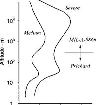
The intensity of the turbulence, represented by the standard deviation or, is a strong function of altitude. We follow Pritchard et al.32 up to 300 m and use the U. S. MIL Standard MIL-A-8866 for higher altitudes. Figure 10.50 depicts two curves.
|
Std. Deviation of Turbulence о – m / s |
The medium profile represents the standard deviation at average gust speeds of 4 m/s, whereas the severe trace centers around 8 m/s. Notice the peak gust velocities in the jet stream of 8 ± 2.3 m/s, which is as much as 20 kn.
To generate time traces from the Dryden spectrum, we have to convert the power spectral density into a filter equation. Driving the filter with white Gaussian noise will produce the desired output. Spectral factorization (see Maybeck33) of Eq. (10.143) yields the transfer function of the gust variable r(s) over the white Gaussian noise vv(v)
r(s) lL/v 1+Уз (L/V)s ic(s)_CrV 2jt (L/V)2s2 +2(L/V)s + 1 For programming we convert the transfer function into its state-space form:
|
X] |
0 |
і |
X] |
0 |
||
|
Xl |
__ Lj |
—– 1 <N 1 |
X2 |
+ |
.(r)2. |
|
r (t) = a |
|
"і V3- |
Xl |
|
v_ |
Xj |
|
L/V 2jt |
You can find these equations programmed in Module G2 of the CADAC GHAME6 simulation. A typical trace is shown in Fig. 10.51. This type of trace r(t) is inserted into the turbulence vector
[uj?]A = [0 0 r]
converted to geographic coordinates with Eq. (10.140), and combined with the wind velocity to be used for the incidence angle calculations in Module G3.
Winds and gusts are important feature of six-DoF simulations. They help us to investigate their effect on the performance, stability, and ride comfort of airplanes. You should be able to model steady winds and turbulence and use the provided data to conduct exploratory studies. For detailed analysis you should comply with the applicable industry standards and consult with the experts of your project team.


