Winds

One of the effects studied in six-DoF simulations is the variability of the atmo­sphere. Air density may deviate from standard conditions, wind and wind shear may dislocate the vehicle, or atmospheric turbulence may shake up the passengers.

In Sec. 8.2.1 I introduced the standard atmosphere and its variations. The in­corporation of wind and turbulence requires the fidelity of six-DoF simulations. Three-DoF and pseudo-five-DoF simulations are inadequate because they do not model incidence angles based on the velocity vector but as output from the auto­pilot.

The air movement over the Earth can be divided into two components. The large – scale horizontal winds and the localized vertical gusts or turbulence. In simulations, tables represent winds as a function of altitude, direction, and magnitude, whereas turbulence, as a random phenomenon, is generated by a stochastic process. We shall discuss both phenomena.

To predict accurately the air movement over the globe is a complex problem. The mathematical model is formulated by partial differential equations and stochastic processes—techniques we would rather dodge. Fortunately, a large database exists of measured wind profiles over the Earth at all seasons, day and night. From this abundance you have to pick the winds that are appropriate for your study. If you have specific locations in mind, the National Oceanographic and Atmospheric Agency (NOAA) will be glad to supply you with archival information.

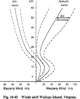
For sensitivity studies you can pick a particular wind profile that is representative of the winds your vehicle may encounter. A reasonable standard is the winds aloft Wallops Island, Virginia, where NASA’s Flight Center is located. Figure 10.45, derived from the Handbook of Geophysics,28 depicts the two extremes, the January and July winds. With little north-south activity it shows only the easterly and westerly components. Taken over many years, the mean winds are plotted against altitude. You can clearly see the jet stream bulges and the severe winds in the stratosphere. I also include a band, one standard deviation wide, to indicate the spread of the data around the mean wind.

You can use Fig. 10.45 or similar plots to define a single wind profile of projected severity, or you can establish an upper bound for winds occurring at a certain probability. For instance, the dashed lines on the right-hand side contain all westerly winds with probability 0.68. If you execute Monte Carlo runs, you can even have the simulation draw the wind profiles from a Gaussian distribution.

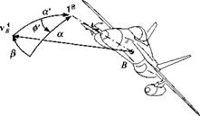
In six-DoF simulations winds and gusts alter the incidence angles and thus change the aerodynamic forces and moments. The incidence angles are calculated from the velocity vector of the vehicle’s c. m. В wrt the air A, expressed in body coordinates ]B, [see Eqs. (3.20-3.23)]. To determine vB, we subtract the wind vector v д from the geographic velocity v § and introduce the body and geographic coordinates and their transformation matrix [T]BG

[vAB]B = [TfG([uf]G – [^]°) (10.139)

Ordinarily, the wind, assumed horizontal, is given by its magnitude Vw and direc­tion from north V’u,. Watch out however for the sign! A north wind blows the air from north to south. In geographic coordinates it has a negative 1G component. Therefore, the wind vector in geographic coordinates is determined by

[vaG = [-Vroc°s jrw – Vu. sin j/w 0]

In CADAC you use the weatherdeck to input winds in tabular form. Go to the G3 Module of the GHAME6 simulation and track down the code that implements Eq. (10.139).