Our heavyweight helicopter equal in the world does not have
In Rostov started production of the most load-lifting rotary-wing car The Russian holding «Helicopt[...]

Everything about aircrafts and helicopters. News and events in aviation worldwide. Civil, transportation, military helicopters and airplanes.

Everything about aircrafts and helicopters. News and events in aviation worldwide. Civil, transportation, military helicopters and airplanes.

Everything about aircrafts and helicopters. News and events in aviation worldwide. Civil, transportation, military helicopters and airplanes.

Everything about aircrafts and helicopters. News and events in aviation worldwide. Civil, transportation, military helicopters and airplanes.


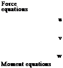
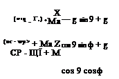
In the following four subsections, analytic expressions for the forces and moments on the various helicopter components are derived. The forces and moments are referred to a system of body-fixed axes centred at the aircraft’s centre of gravity/mass, as illustrated in Fig. 3.1. In general, the axes will be oriented at an angle relative to the principal axes of inertia, with the x direction pointing forward along some convenient fuselage reference line. The equations of motion for the six fuselage DoFs are assembled by applying Newton’s laws of motion relating the applied forces and moments to the resulting translational and rotational accelerations. Expressions for the inertial velocities and accelerations in the fuselage-fixed axes system are derived in Appendix Section 3A.1, with the resulting equations of motion taking the classic form as given below.
 |
|
 |
|
|
|
![]()
![]() hxp = (Iyy — Izz) qr + Ixz (r + pq) + l
hxp = (Iyy — Izz) qr + Ixz (r + pq) + l
Iyyq = (Izz — Ixx) rp + Ixz (r2 — p2) + M Izzr = (Ixx — Iyy) pq + Ixz( p — qr) + N
where u, v and w and p, q and r are the inertial velocities in the moving axes system; ф, 9 and ф are the Euler rotations defining the orientation of the fuselage axes with respect to earth and hence the components of the gravitational force. Ixx, Iyy, etc., are the fuselage moments of inertia about the reference axes and Ma is the aircraft mass. The external forces and moments can be written as the sum of the contributions from the different aircraft components; thus, for the rolling moment
L = LR + LTR + L f + Ltp + Lfn (3.7)
where the subscripts stand for: rotor, R; tail rotor, TR; fuselage, f; horizontal tailplane, tp; and vertical fin, fn.
In Chapters 4 and 5, we shall be concerned with the trim, stability and response solutions to eqns 3.1-3.6. Before we can address these issues we need to derive the expressions for the component forces and moments. The following four sections contain some fairly intense mathematical analyses for the reader who requires a deeper understanding of the aeromechanics of helicopters. The modelling is based essentially on the DRA’s first generation, Level 1 simulation model Helisim (Ref. 3.4).
A few words on notation may be useful before we begin. First, the main rotor analysis is conducted in shaft axes, compared with the rotor-aligned, no-flapping or nofeathering systems. Appendix Section 3A.5 gives a comparison of some expressions in the three systems. Second, the reader will find the same variable name used for different states or parameters throughout the chapter. While the author accepts that there is some risk of confusion here, this is balanced against the need to maintain a degree of conformity with traditional practice. It is also expected that the serious reader of Chapters 3, 4 and 5 will easily cope with any potential ambiguities. Hence, for example, the variable r will be used for rotor radial position and aircraft yaw rate; the variable в will be used for flap angle and fuselage sideslip angle; the variable w will be used for blade displacement and aircraft inertial velocity along the z direction. A third point, and this applies more to the analysis of Chapters 4 and 5, relates to the use of capitals or lowercase for trim and perturbation quantities. For the work in the later modelling chapters we reserve capitals, with subscripts e (equilibrium), for trim states and lowercase letters for perturbation variables in the linear analysis. In
|
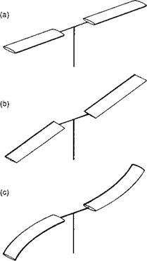
Fig. 3.4 Three flap arrangements: (a) teetering; (b) articulated; (c) hingeless |
Chapter 3, where, in general, we will be dealing with variables from a zero reference, the conventional lowercase nomenclature is adopted. Possible ambiguities arise when comparing analysis from Chapters 3, 4 and 5, although the author believes that the scope for confusion is fairly minimal.