Multi-blade coordinates

We can introduce a transformation from the individual blade coordinates (IBCs) to the disc coordinates, or multi-blade coordinates (MBCs), as follows:

(3.49)

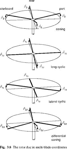
Once again, the reference zero angle for blade 1 is at the rear of the disc. The MBCs can be viewed as disc mode shapes (Fig. 3.8). The first, во, is referred to as coning – all the blades flap together in a cone. The first two cyclic modes в1с and e1s represent first harmonic longitudinal and lateral disc tilts, while the higher harmonics appear as a disc warping. For Nb = 4, the oddest mode of all is the differential coning, Pod, which can be visualized as a mode with opposite pairs of blades moving in unison, but

in opposition to neighbour pairs, as shown in Fig. 3.8. The transformation to MBCs has not involved any approximation; there are the same number of MBCs as there are IBCs, and the individual blade motions can be completely reconstituted from the MBC motions. There is one other important aspect that is worth highlighting. MBCs are not strictly equivalent to the harmonic coefficients in a Fourier expansion of the blade angle. In general, each blade will be forced and will respond with higher than a one-per-rev component (e. g., two-, three – and four-per-rev), yet with Nb = 3, only first harmonic MBCs will exist; the higher harmonics are then folded into the first harmonics. The real benefit of MBCs emerges when we conduct the coordinate transformation on the uncoupled individual blade eqns 3.34, written in matrix form as
hence forming the MBC equations

Pm + cm ІФ )P’M + Dm ІФ )Pm = Hm ІФ) (3.51)

where the coefficient matrices are derived from the following expressions:

Cm = Ь-1|2Ц + C i LeJ	(3.52)
= L-1 j Le+ Ci Vp + D i Lej	(3.53)
Hm = L-1Hi	(3.54)

Dm

The MBC system described by eqn 3.51 can be distinguished from the IBC system in two important ways. First, the equations are now coupled, and second, the periodic terms in the coefficient matrices no longer contain first harmonic terms but have the lowest frequency content at Nb/2 per-rev (i. e., two for a four-bladed rotor). A common approximation is to neglect these terms, hence reducing eqn 3.51 to a set of ordinary differential equations with constant coefficients that can then be appended to the fuse­lage equations of motion allowing the wide range of linear stationary stability analysis tools to be brought to bear. In the absence of periodic terms, MBC equations take the form

Pm + Cm 0PM + Dm 0Pm = Hm 0(f) (3.55)

where the constant coefficient matrices can be expanded, for a four-bladed rotor, as shown below:

(3.56)

)

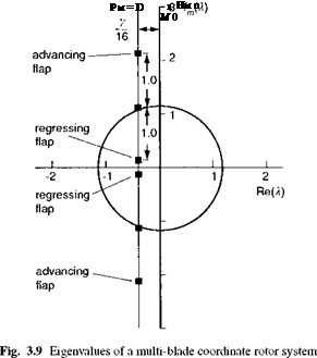
The two modes have been described as the flap precession (or regressing flap mode) and nutation (or advancing flap mode) to highlight the analogy with a gyroscope; both have the same damping factor as the coning mode but their frequencies are widely separated, the precession lying approximately at X – 1) and the nutation well beyond this at (Xe + 1). While the nutation flap mode is unlikely to couple with the fuselage motions, the regressing flap mode frequency can be of the same order as the highest frequency fuselage modes. An often used approximation to this mode assumes that the inertia terms are zero and that the simpler, first-order formulation is adequate for describing the rotor flap as described in Chapter 2 (eqn 2.40). The motion tends to be more strongly coupled with the roll axis because of the lower time constant associated with roll than with pitch motion. The roll to pitch time constants are scaled by the ratio of the roll to pitch moment of inertia, a parameter with a typical value of about 0.25. We shall return to this approximation later in this chapter and in Chapter 5.

The differential coning is of little interest to us, except in the reconstruction of the individual blade motions; each pair of blade exerts the same effective load on the rotor hub, making this motion reactionless. Ignoring this mode, we see that the quasi-steady motion of the coning and cyclic flapping modes can be derived from eqn 3.55 and written in vector-matrix form as

or expanded as

вм = Ape 0 + ApxX + Арыш (3.65)

where the subvectors are defined by

вм = {во, Ріс, Pis} (3.66)

0 ={{0, etw-l eisw 7 eicw } (3.67)

X = {(Д^ — ^0)7 ^1sw 7 Xicw } (3.68)

W = {p’hw 7 qhw 7 Phw 7 qhw } (3.69)

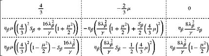
and the coefficient matrices can be written as shown opposite in eqns 3.70, 3.71 and 3.72. Here

1

1 + SP

These quasi-steady flap equations can be used to calculate rotor trim conditions to O(p? ) and also to approximate the rotor dynamics associated with low-frequency fuselage

(3.70)

(3.71)

2

(3.72)

motions. In this way the concept of flapping derivatives comes into play. These were introduced in Chapter 2 and examples were given in eqns 2.29-2.32; the primary flap control response and damping in the hover were derived as

dP1c	dPls	1
d$1s	ddic	1 +
d^ls	1	L 16
д p	1 + Sj	Sf + 7)

dfitc d q

showing the strong dependence of rotor flap damping on Lock number, compared with the weak dependence of flap response due to both control and shaft angular motion on rotor stiffness. To emphasize the point, we can conclude that conventional rotor types from teetering to hingeless, all flap in much the same way. Of course, a hingeless rotor will not need to flap nearly as much and the pilot might be expected to make smaller control inputs than with an articulated rotor, to produce the same hub moment and hence to fly the same manoeuvre.

The coupled rotor-body motions, whether quasi-steady or with first – or second – order flapping dynamics, are formed from coupling the hub motions with the rotor and driving the hub, and hence the fuselage, with the rotor forces. The expressions for the hub forces and moments in MBC form will now be derived.