Our heavyweight helicopter equal in the world does not have
In Rostov started production of the most load-lifting rotary-wing car The Russian holding «Helicopt[...]

Everything about aircrafts and helicopters. News and events in aviation worldwide. Civil, transportation, military helicopters and airplanes.

Everything about aircrafts and helicopters. News and events in aviation worldwide. Civil, transportation, military helicopters and airplanes.

Everything about aircrafts and helicopters. News and events in aviation worldwide. Civil, transportation, military helicopters and airplanes.

Everything about aircrafts and helicopters. News and events in aviation worldwide. Civil, transportation, military helicopters and airplanes.


Consider the computation of the solution of the nonlinear simple wave equation (8.12) by a high-order finite difference scheme. For this purpose, it is more convenient to use dimensionless variables with mesh size Ax as the length scale, speed of sound a0 as the velocity scale, and Ax/a0 as the time scale. On recasting (8.12) into a conservation form, the initial value problem is
![]() д u д u y + 1 д u2
д u д u y + 1 д u2
—– 1—— + —л——– = 0
д t д x 4 дx
|
3 , 1 3 a u{n) – Y + 1 aiuj+t 4 |
 |
Consider the initial condition in the form of a Gaussian function as follows:
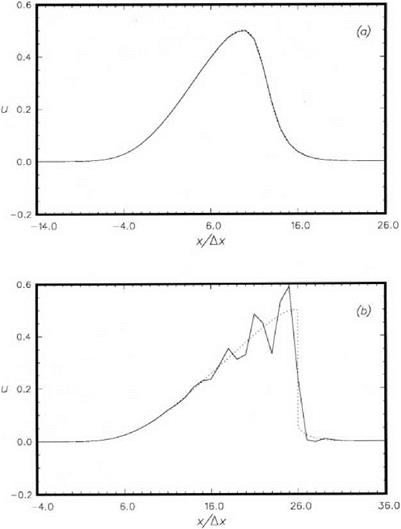
The solution of Eq. (8.19) with initial condition (8.21) can be computed easily. Figure 8.2 shows the computed results for the case h = 0.5 and b = 5.0 at t = 6 and t = 16. At t = 6, the waveform, unlike the initial shape, is no longer symmetric about its maximum. It has been substantially distorted by nonlinear steepening effects. The waveform is in good agreement with the exact solution. t = 6 is very near to the wave breaking time when a shock will form.
At t = 16, a shock has formed in the exact solution. Clearly, the high-order finite difference scheme cannot reproduce a sharp discontinuity. The shock is replaced by a steep gradient. However, following the steep gradient are spurious spatial oscillations. The presence of these spurious oscillations renders the numerical solution totally unacceptable.
The spurious oscillations are not related to the Gibbs phenomenon as many investigators had speculated. What causes the spurious spatial oscillations then? It turns out that a good deal of the understanding of the origin of the spurious oscillations can be found by studying and comparing the time evolution of the exact and finite difference solutions in wave number space.
|
33 EY + 1 , ,2 ajuj+i + E aj(uj+i) j=-3 4 j=-3 |
 |
||
The Fourier transform of Eq. (8.17) and initial condition (8.20) is
|
This is a special case of the following finite difference differential equation in which x is a continuous variable.
3 3
d lu (x t ) y + 1
![]()
![]() ’ + ^2 aju (x + i^x, t) + ^—4— ^2 aju2 (x + j&x, t) = 0. (8.25)
’ + ^2 aju (x + i^x, t) + ^—4— ^2 aju2 (x + j&x, t) = 0. (8.25)
i=-3
The Fourier transform of Eq. (8.25) is
where a (a ) is the wave number of the finite difference scheme.
Both Eqs. (8.22) and (8.26) with initial condition (8.23) describe the time evolution of a nonlinear acoustic pulse in wave number space. Eq. (8.22) is for the exact
solution. Eq. (8.26) is for the finite difference equation. These nonlinear integral- differential equations can be solved numerically by first discretizing the wave number axis into a fine mesh of spacing Да. The integrals are then converted to sums. This reduces the equation to a system of (2M + 1) first-order ordinary differential equations in time, where M is a large integer.
Eqs. (8.22) and (8.26) become, upon discretizating the а-axis,
where т = – M, – M + 1,…, M, and, U j = U j = 0 if j > M. The initial condition is
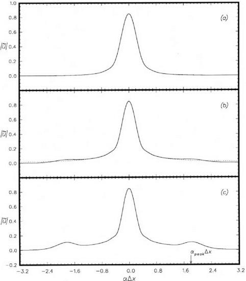
The systems of Eqs. (8.27) and (8.28) with initial condition (8.29) can be integrated in time numerically by the Runge-Kutta method. The computed results are shown in Figure 8.3 for the case h = 0.5 and b = 5.0. The time evolution of the pulse in physical space is given in Figure 8.2. At t = 6, the wave number spectrum is smooth and nearly Gaussian as shown in Figure 8.3a. There is very little difference between the exact and the finite difference solution. At t = 11.67, the shock formation time, the wave number spectra are shown in Figure 8.3b. The computed and the exact wave number spectra are no longer identical. A small spurious peak appears at а Дх = 1.8 for the finite difference solution. This peak grows in height as time progresses. At time t = 16, a significant peak has developed as can be seen in Figure 8.3c.
In the physical space, Figure 8.2b, the dominant wavelength of the spurious spatial oscillations is about 3.5Дх. The corresponding wave number is аДх = — 1-8.
Clearly, the accumulation of wave energy around the spurious peak in the wave number space is the cause of the appearance of the extraneous spatial oscillations in the waveform in physical space. Let us now determine the factors that could significantly influence the wave number at the maximum of the spurious peak, namely, а^. A list of the likely factors is as follows:
1. The initial waveform of the acoustic pulse.
2. Whether the equation is cast in conservation form or nonconservation form.
3. The size of the finite difference stencil, N.
To test the effect of the initial waveform, the following families of initial profile shapes will be considered.
(a) Gaussian Profile
|
(b)
 |
|
The Lorentz Line Shape
Each of these waveforms is characterized by two parameters, namely, h (the maximum amplitude) and b (the half-width). For each initial waveform, the systems
where к(k) is a (a) with a ^ k, is integrated in time. The location apeak Ax in wave number space using stencil size N = 3,5, and 7 are determined computationally. The results are given in Figures 8.4a, 8.4b, and 8.4c. These results suggest the following conclusions.
1. Whether the governing partial differential equation is cast in conservation form or not has only a minor effect on the location of apeak Ax.
2. The initial profile shape of the waveform has a stronger influence than whether the equation is in conservation form or not.
3. The stencil size has the dominant influence. The value of apeak Ax shifts to higher values with increase in stencil size.
A different presentation of this result is given in Figure 8.5. It is found that apeakAx invariably lies in the range marked AB in the a Ax versus a Ax plot. Two other important points are observed. (a) Point A is nearly equal to ac Ax so that the wave number of the spurious spectrum peak is definitely in the short wave range. (b) apeakAx lies close to where a Ax is largest. It is not difficult to understand these results. The term и(ди/дx) or 1/2(дu2/Bx) in the partial differential equation is the nonlinear steepening term. It causes the solution to cascade to finer and finer scales or higher wave numbers. For the finite difference scheme, the nonlinear term in wave number space is
(Ю
a j їй (k, t) U (a — k, t )dk
— TO
This is weighted by a so that it favors the transfer of energy to wave numbers for which a is the largest.
Once energy cascades into this wave number range, further cascading is prevented by the dispersive nature of the numerical waves. Dispersive waves propagate with different wave speeds. This reduces the effectiveness of nonlinear interaction and hence the cascading process. This is why the wave energy piles up around wave number apeak Ax without cascading to even higher wave numbers.