Variable Artificial Selective Damping

Now the origin of the spurious spatial oscillations around a computed shock solution is known; what is needed to obtain an acceptable nonlinear solution is to eliminate the short waves around the peak at a Ax = apeak Ax. One way to do this is to use artificial selective damping, which was discussed in Chapter 7. For a nonlinear wave

propagation problem, artificial selective damping is needed only in the limited region of space where large gradients occur. The use of a constant artificial viscosity, which introduces uniform damping everywhere, is not a good strategy. For a high-quality numerical solution, the use of a variable artificial viscosity or mesh Reynolds number is desirable.

To establish a variable damping algorithm, a way to measure the shock strength or velocity gradient is needed. A shock is expected to be smeared out over a few mesh points, so the relevant measure of length is Ax (the mesh size). As a measure of velocity, one may use wstencil = |wmax – wmin|; the difference between the maximum velocity, wmax, and the minimum velocity, wmin, within the stencil. Note: if a very large stencil is used in the finite difference scheme, one might consider restricting

the determination of umax and umin to a smaller substencil in forming ustencil. It is useful to define a stencil Reynolds number, Rstencil, by

Rstencil = UstefAX. (8.34)

On adding artificial selective damping terms to the discretized nonlinear simple wave equation (8.12), it is straightforward to find (in dimensional form) the following:

In Eq. (8.35), the ratio of the magnitude of the nonlinear steepening term to the damping term is (Note: velocity scale is ustencil) as follows:

So Rstencil may be interpreted as the rate of generation of spurious short waves around a Ax = apeak Ax to the rate of removal of the short waves by artificial selective damping. What one would like to see is that, as soon as the spurious waves are

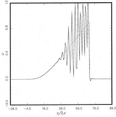
Figure 8.6. Computation of nonlinear acoustic pulse without artificial damping. t = 36. Gaus­sian initial waveform with h = 1.0, b = 12 Ax.—————————————————————- , computed,…………. exact solution.

generated, they are eliminated by damping. In other words, the generation and damping processes are matched or balanced. This means that ^stencil is a universal constant. Here, a universal constant means that it is independent of the nonlinear problem to be solved. However, the value of the constant obviously depends on the damping curve and the finite difference scheme being used.

To find ^stencil for the 7-point stencil DRP scheme and a damping curve of half­width 0.3n, extensive numerical experiments have been carried out. It is found that by taking ^stencil — 0.06 to 0.1 most of the preshock and postshock spurious spatial oscillations are removed from the numerical solutions for all the initial pulse profiles that have been considered.

Two numerical examples are provided here. Figure 8.6 shows the computed waveform at t = 36 (in Ax/a0 units) when no artificial selective damping terms are included. The initial pulse profile is a Gaussian with h = 1.0 and b = 12. The waveform is clearly dominated by spurious spatial oscillations bearing little resemblance to the exact solution. Figure 8.7 is the computed solution with artificial selective damping terms. ^stencil is set at 0.1 (for general application, ^stencil = 0.06 gives the best overall results). The numerical solution compares favorably with the exact solution with a fitted shock according to the Whitham (1974) method. Figure 8.8 shows the case with h = 0.5 and b = 3. At t = 72 the numerical solution without artificial selective damping consists of random spikes. The computed results seemingly have no relationship to

result with variable damping (Rstencil = 0.1). The computed shock matches well with the exact solution. The shock is smeared out approximately over five mesh spacings.

Concerning whether one should put the governing equations of gas dynamics in a conservation form before computing the solution using the variable damping method for shock capturing, extensive testing indicates that this is a requirement if an accurate solution is to be obtained. Test results reveal that the use of governing equations in nonconservation form often leads to a slower propagation shock. This is, perhaps, not altogether surprising since in gas dynamics the shock speed depends on the conservation of mass, momentum, and energy across the shock.

EXERCISES

8.1.

The inviscid Burger’s equation can be written in a conservation or nonconser­vation form

Solve these equations computationally using the variable damping method with the initial condition,

t = 0 u = 0.5e~(ln2)( 5)

where Ax = 1.

Assess the accuracy of the two solutions, especially the location of the shock as a function of time by comparing the solutions with the shock-fitted solution following Whitham’s equal area rule (see Whitham (1974) section 2.8).

8.2.

Solve the simple nonlinear wave equation,

with initial condition, t = 0

21

by adding variable damping to the numerical scheme. Compare the solutions obtained using a 7-point stencil and a 15-point stencil (using the same size damping stencil as the computation algorithm). Compare the time history of the shock with that obtained by Witham’s equal area rule.

8.3. In dimensionless form with respect to the following scales:

length scale = Ax velocity scale = aref time scale = Ax/aref density scale = pref pressure scale = pref.

the Euler equations in one dimension are

where E = . p 1 u2.

(Y-1)p 2

Solve the shock tube problem using the following initial conditions and a com­putation domain -100 < x < 100, t = 0, u = 0:

	, x < -2
4.4 ( ((x + 2) n 2.7 + 1.7 cos 1—— 4—–	-2 < x < 2
1	, x > 2
p = (YP)1/Y, Y	= 1.4.

p=

Find the spatial distribution of p, p, and u at t = 40, 50, 60, and 70. Compare your numerical solution with the standard shock tube solution.